Feed-Forward Neural Networks Presentation

I was asked to give a presentation on feed-forward neural networks for a deep learning study group. This was largely based on the Deep Learning Book (chapter 6) aswell as the CS231n course, the coursera courses, Machine Learning and Neural Networks and Deep Learning. My slides are below along with notes.

In previous presentations given by others the group had quickly covered some basic machine learning techniques including linear regression. I started by recapping this.

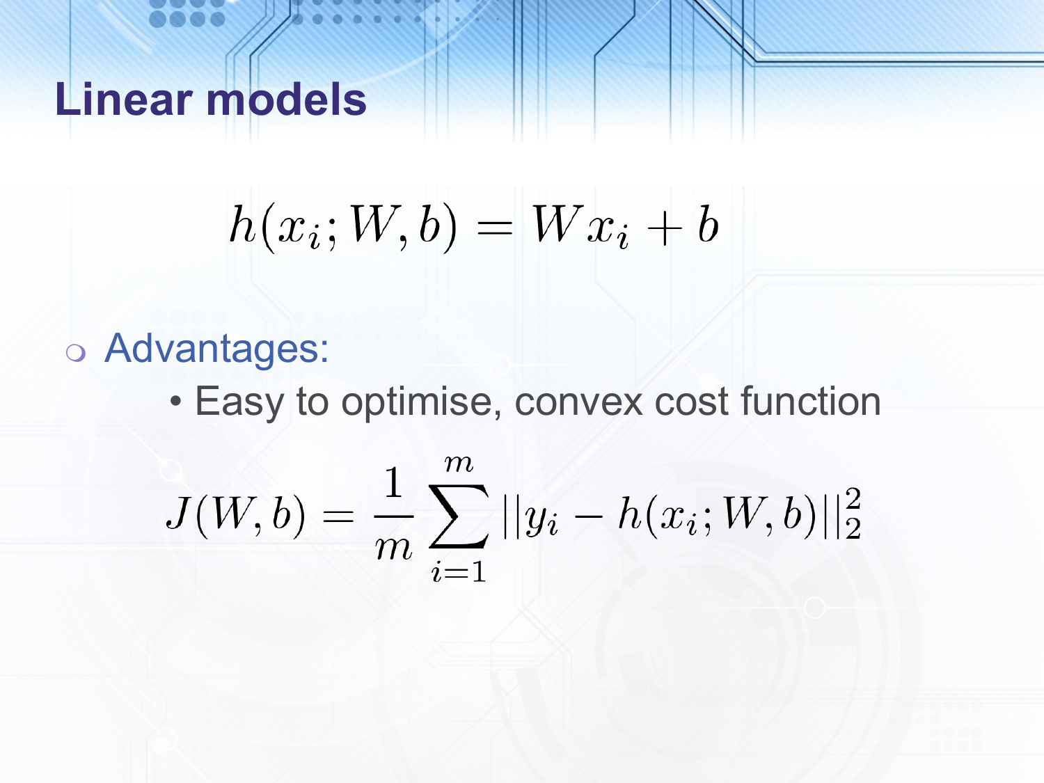
For each input data point $x_i$ our hypothesis, $h$, is a linear transformation of the input. We use the mean squared error as our cost function which is easy to optimise using for example gradient descent since it is convex and therefore we can guarantee not to get stuck in a local minimum (or saddle point).

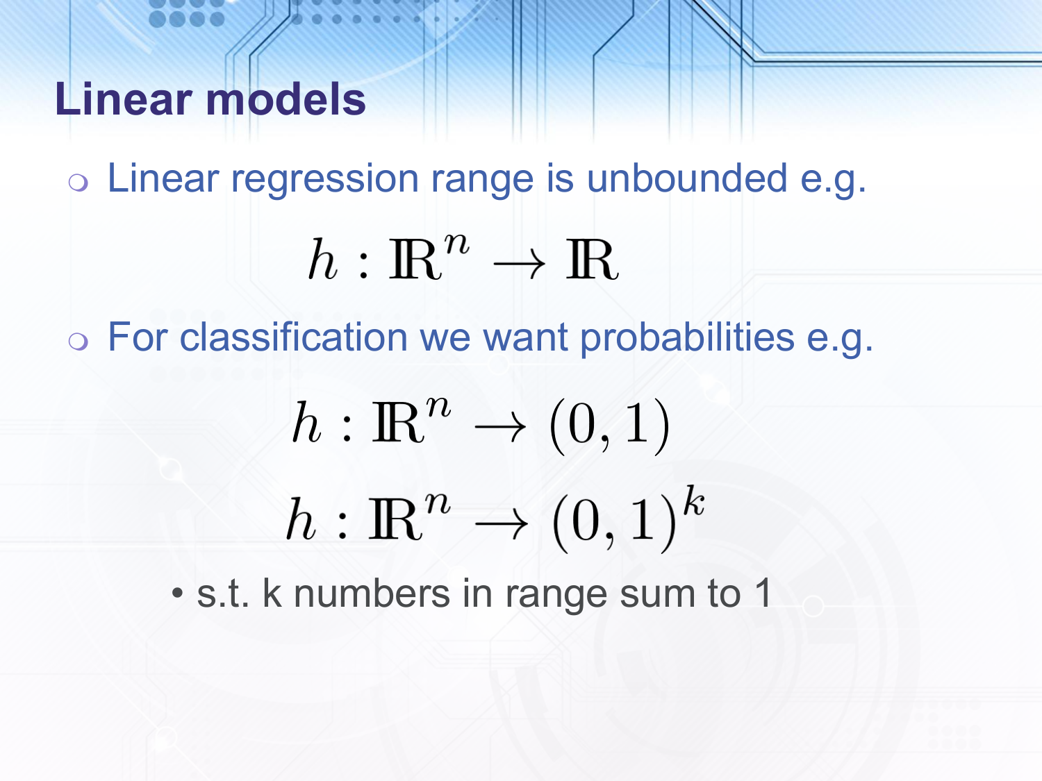
As a function approximation technique, the output of linear regression is unbounded i.e. it is in $\mathbb{R}$ or $\mathbb{R}^k$. However, for classification tasks this does not work well. For example, if we have a binary classification problem, so the $y_i$ values are $0$ or $1$, the output of linear regression will only be close to $0$ and $1$ briefly and then continue increasing or decreasing as we get further from the dividing line. This increases the cost of points which are already on the correct side of the line. We can improve the situation by having a function which gets closer to $1$ as we get further to one side of the line and closer to $0$ on the other side. This implies that for binary classification the range of our hypothesis should be $(0, 1)$. In some sense this could be considered as our hypothesis estimating the probability of $x_i$ being a positive example. For multi-class classification with $k$ classes, it turns out that the hypothesis we use for binary classification can be extended to $k$ dimensions. We normalise to ensure that the numbers output sum to $1$ so that we can continue with our interpretation of the hypothesis output being the probability per class.

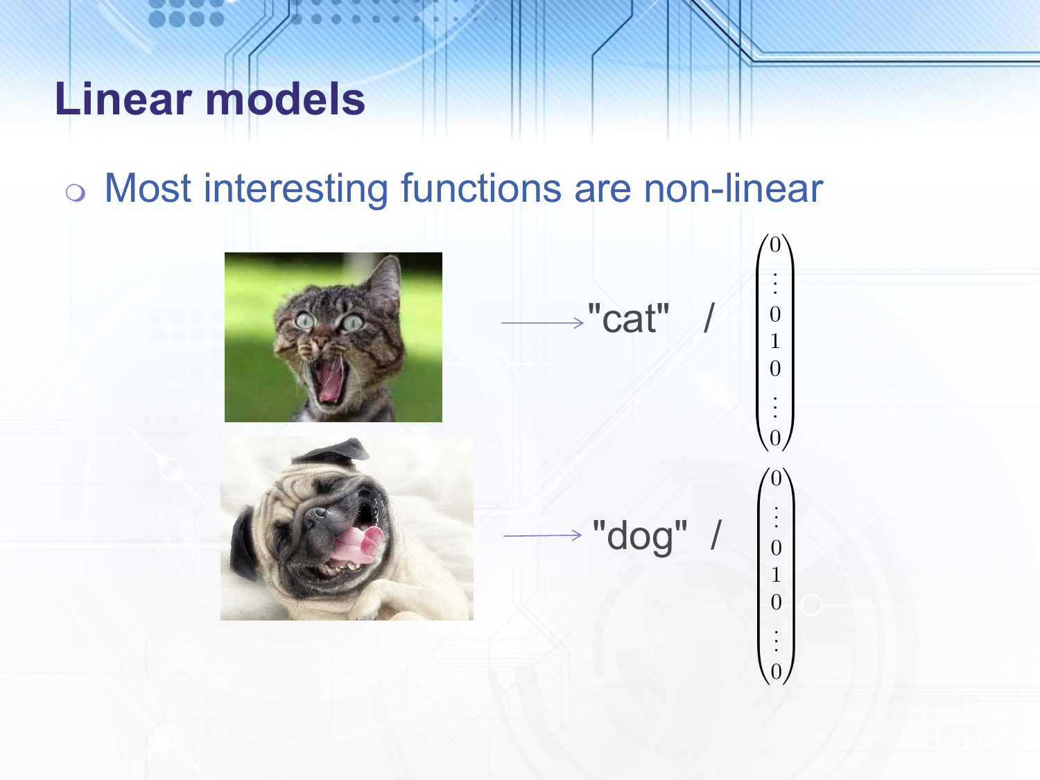
Another problem with linear regression is that most interesting functions are non-linear. This can be seen by visualising examples from tasks such as object recognition. This can also be seen when we apply a linear model with a convex cost function to difficult problems such as object recognition and get poor performance. If we can show that we have converged to a local minimum then we must also be at a global minimum of the cost function. If the cost function is reasonable then for linearly separable classes we should get very good performance.

To address the issue of the unbounded output range we can use logistic or softmax regression.

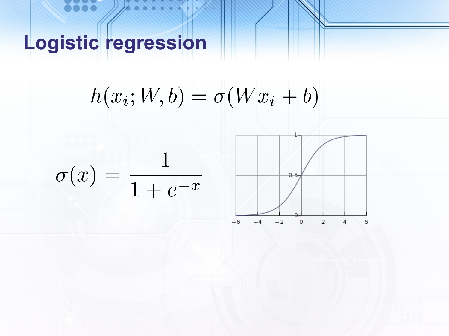
In logistic regression we first do a linear transformation of the input data $x_i$ and then apply the logistic sigmoid function, which is shown in the slide. As discussed above this has the desirable property of asymptotically reaching $1$ as the input (i.e. the result of the linear transformation) tends to $\infty_+$ and $0$ as the input tends to $\infty_-$.

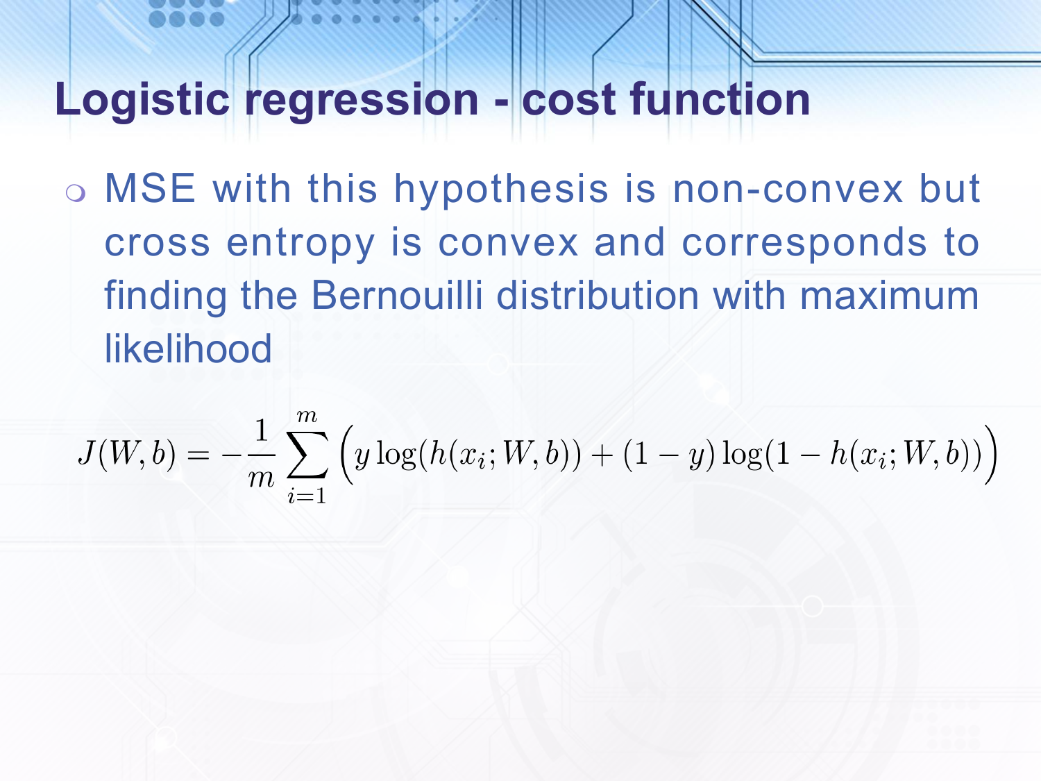
If we use the same mean squared error cost function that we did with linear regression the result would be non-convex. Instead we use the cross entropy which is convex and will converge on the maximum likelihood distribution.

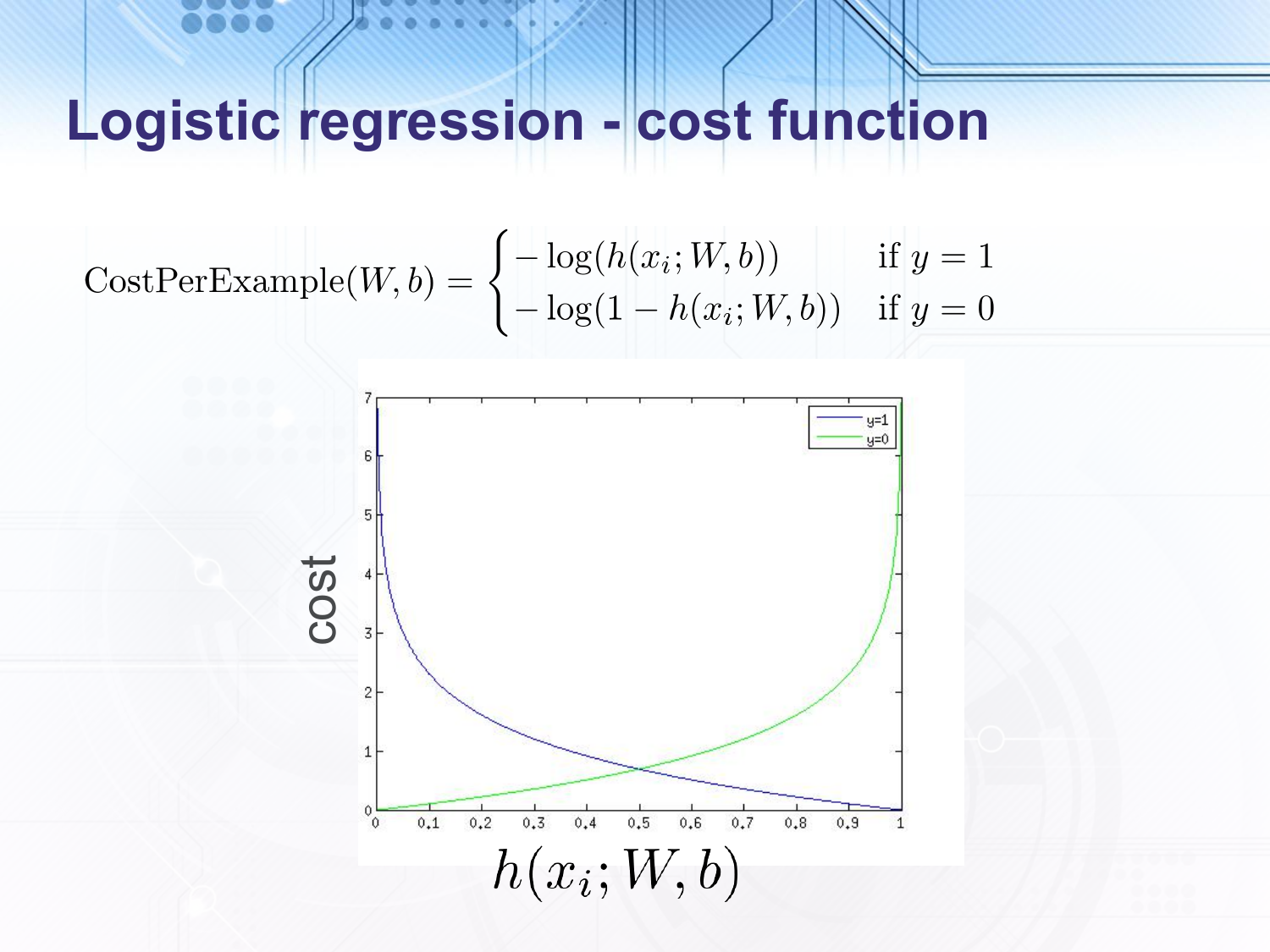
Intuitively, the cost per example goes to $0$ when the hypothesis for the example is close to the correct classification and goes to $\infty$ when the hypothesis is close to the incorrect classification.

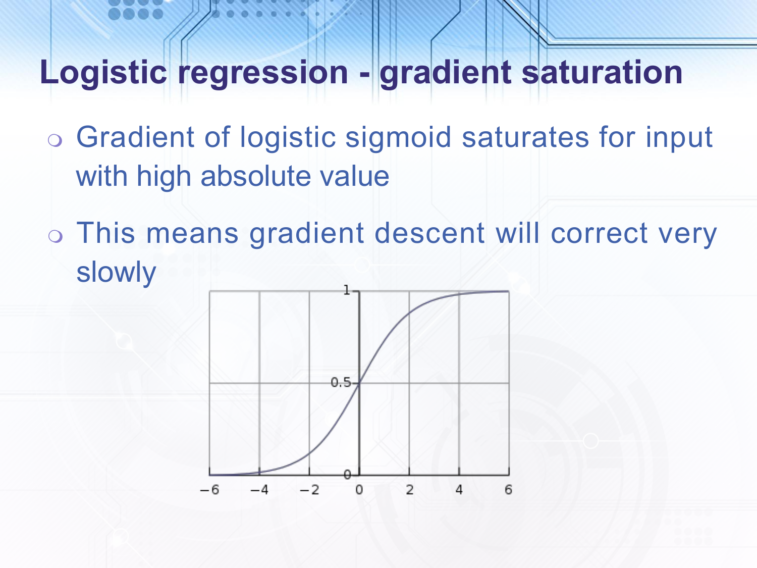
The gradient of the logistic sigmoid asymptotically reaches $0$ when the input is far from $0$, so if we were using something like mean squared error for our cost function it would correct very slowly when the input to the logisitc sigmoid is very far to one side, even if it is the incorrect side.

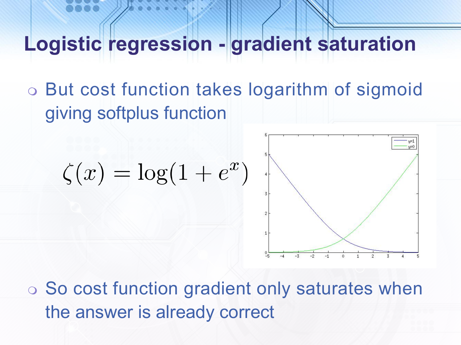
However, with our cross entropy function we do not have this issue since we take the logarithm of the sigmoid and get something called the softplus function, which is shown in the slide. The gradient of the softplus only saturates when the input to the logistic sigmoid is very far on the correct side of the line i.e. when we already have the answer correct. When the input is far to the incorrect side of the line the gradient is approximately linear.

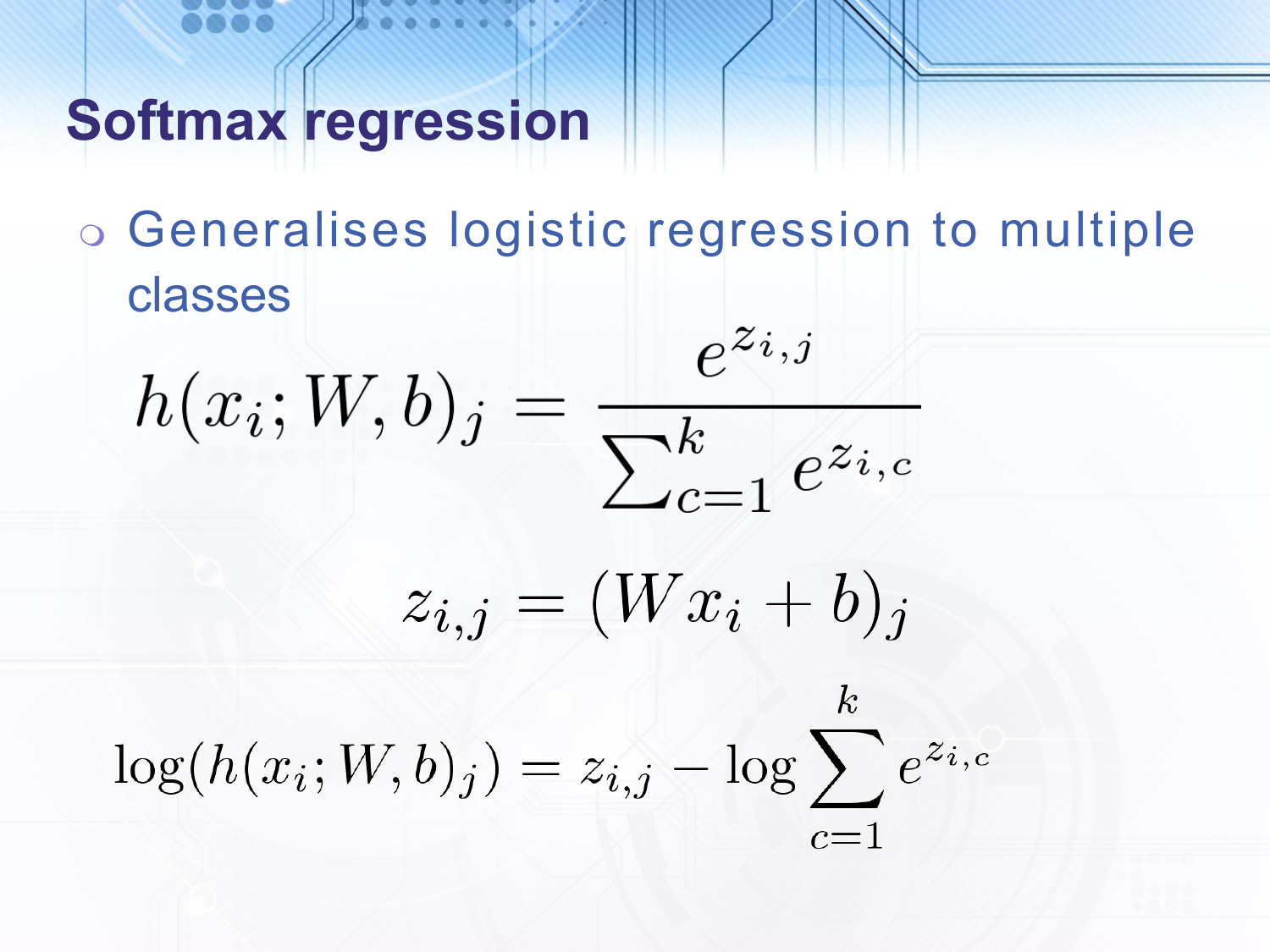
Softmax regression is the generalisation of logistic regression to a multidimensional output. We start by applying a linear transformation which has a multidimensional output. We then take the exponent of each element in the vector and normalise. To see that this is a generalisation of logistic regression first note that $\frac{1}{1 + e^{-x}} = \frac{e^x}{1 + e^{x}}$. Next note that if we output $k$ numbers for $k$ classes then we have overparameterised the problem, since the constraint that the numbers sum to 1 means that once we have chosen $k - 1$ numbers we have no choice about the last. To avoid the overparameterisation we could specify $z_{i,k} = 0$, this would then give a hypothesis for the remaining classes of $\frac{e^{z_{i,j}}}{1 + \sum_{c=1}^{k-1}e^{z_{i,c}}}$. In the case where $k = 2$ this reduces to the logistic sigmoid. In practice, it tends not to matter whether we use the overparameterised version and therefore this is normally used for simplicity.

Also, note that the logarithm of the hypothesis is the linear transformation of the $j^{\mathrm{th}}$ class minus the log of the sum of exponents for all classes, this will come up later as we evaluate the effect of gradient descent on the cost function.

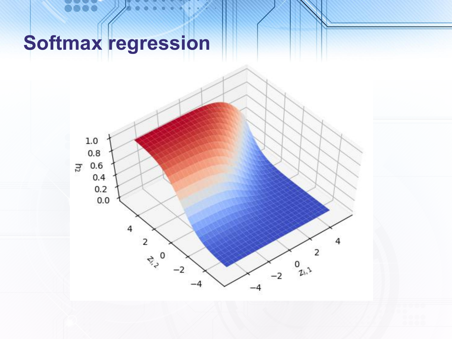
In the above slide, I have plotted the output of the correctly parameterised version of softmax regression (i.e. where $z_{i,k}$ is set to 0) for a 3 class output. On two of the axes we show $z_{i,1}$ and $z_{i,2}$ (remember $z_{i,3} = 0$). Then on the third axis we show the output of the second class, $h_2$. As you can see $z_{i,2}$ has to be much greater than 0 and much greater than $z_{i,1}$ to get a value close to 1. In logistic regression the input must just be much greater than $0$, whereas in softmax regression the input must be much greater than all of the other inputs.

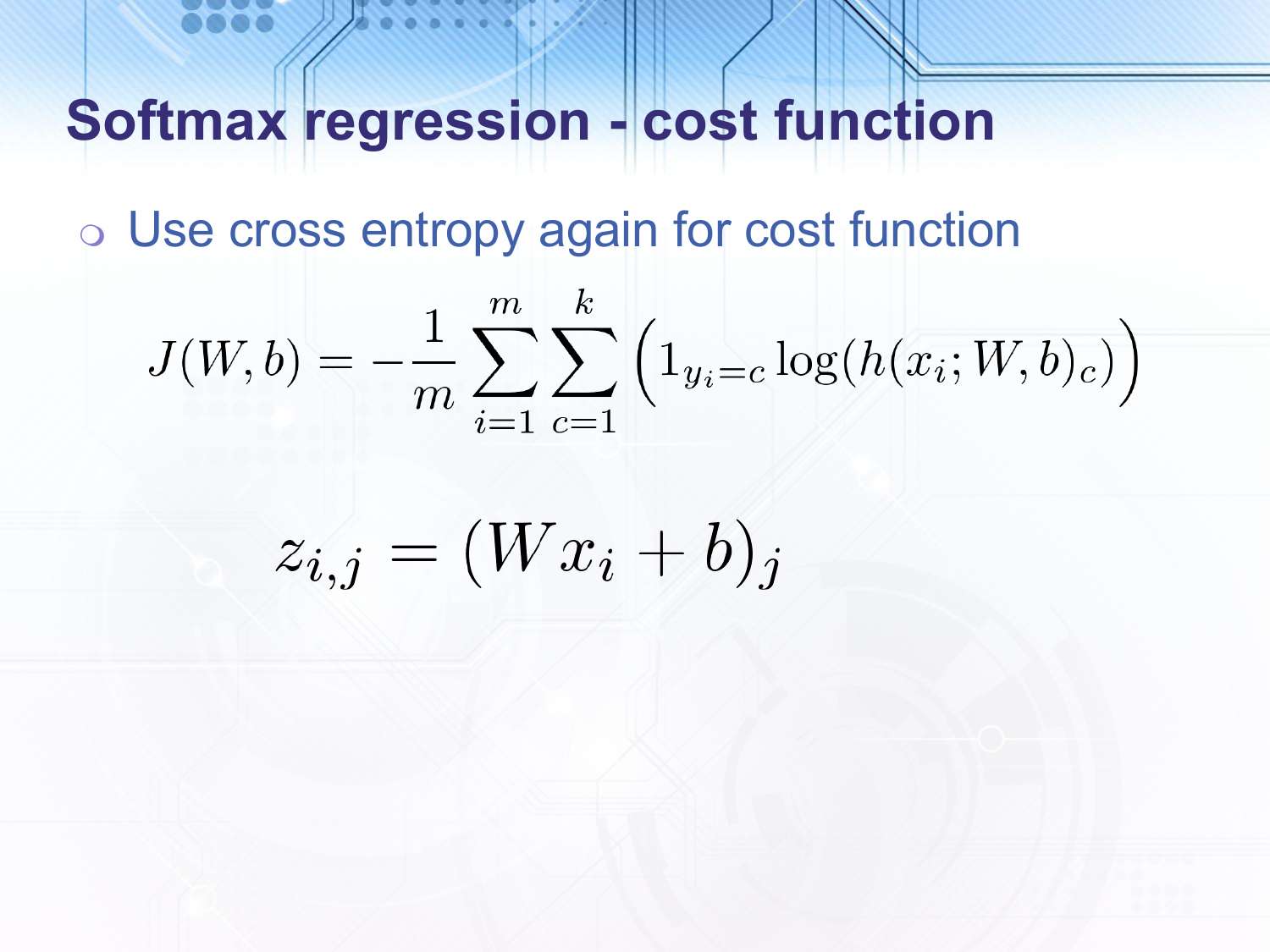
As with logistic regression, we use the cross entropy cost function which is again convex and again will converge on the maximum likelihood distribution.

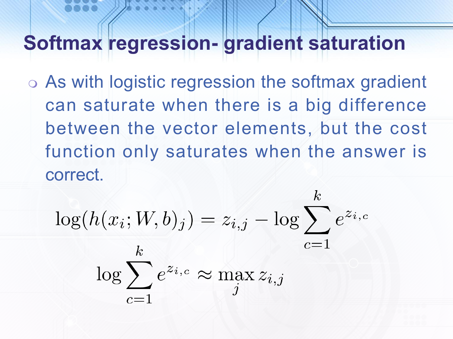
As with logistic regression, the softmax gradient saturates when the inputs are very different even if the highest input is the wrong class. But by taking the logarithm in the cost function we get a similar situation to the softplus function. Unfortunately I didn’t put this in the slides but I will add here a plot of the cost per example for $h_2$.

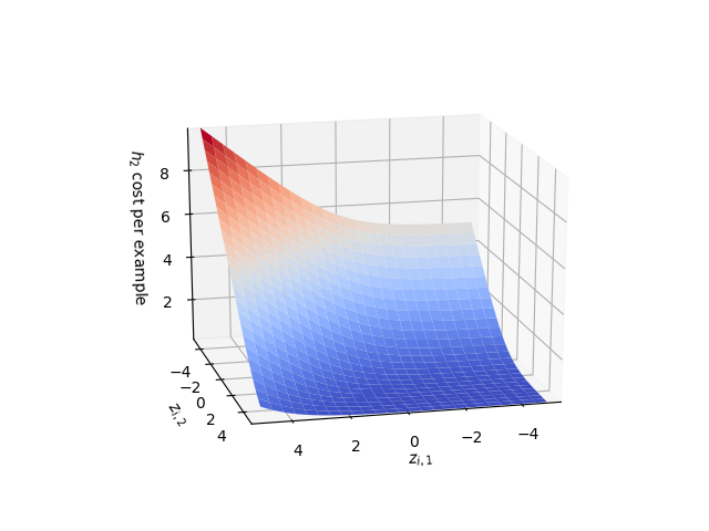
As you can see in the figure the gradient of this is approximately linear when $z_{i,2}$ is much less than $0$ or $z_{i,1}$ and saturates when it is much greater than both i.e. when the answer is correct.

Another way to see why this is the case is to note that when $z_{i,j}$ is much greater than all of the other $z_{i,c}$ then $\mathrm{log} \sum_{c=1}^k e^{z_{i,c}} \approx \max_{j} z_{i,j}$, so if the correct input is much greater than the other inputs then the log of the hypothesis is approximately $0$ otherwise the log is approximately the correct input minus the largest incorrect input.

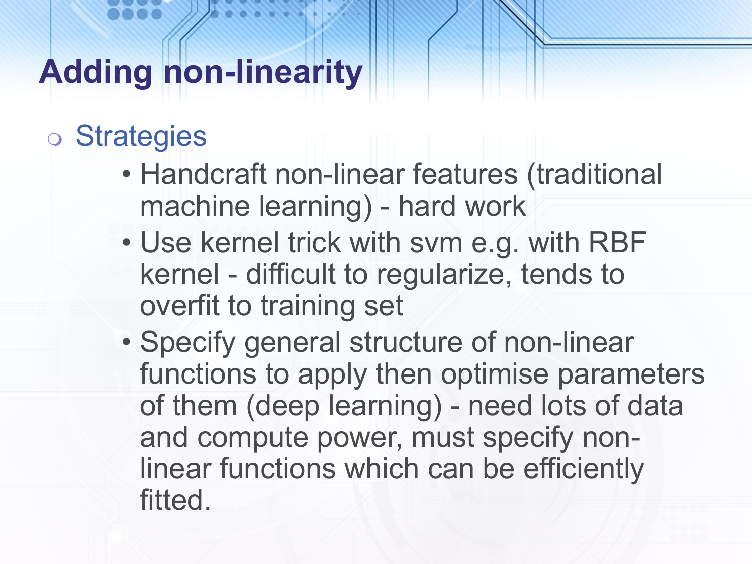
Now, to deal with the second problem with linear regression we need to add non-linearity, i.e. to transform the input data points in a non-linear way such that the results are now linearly separable. In traditional machine learning the most effective technique was to handcraft non-linear transformations to apply to the input data. This included things like histograms of oriented gradients in patches of an image. The biggest problem with this was that people could work for decades on a small application area trying to come up with better non-linear transformations. There was also a popular technique to create non-linear transformations by adding a radial basis function kernel at each input data point, however this would overfit the training data. The approach of deep learning is to specify the general structure of some non-linear transformations and then optimise the parameters of them. This is very successful but requires a lot of data and computation and since the resulting cost function that we use is non-convex we must be careful in specifying the types of non-linear transformations that we use to ensure that optimisation strategies such as gradient descent will work.

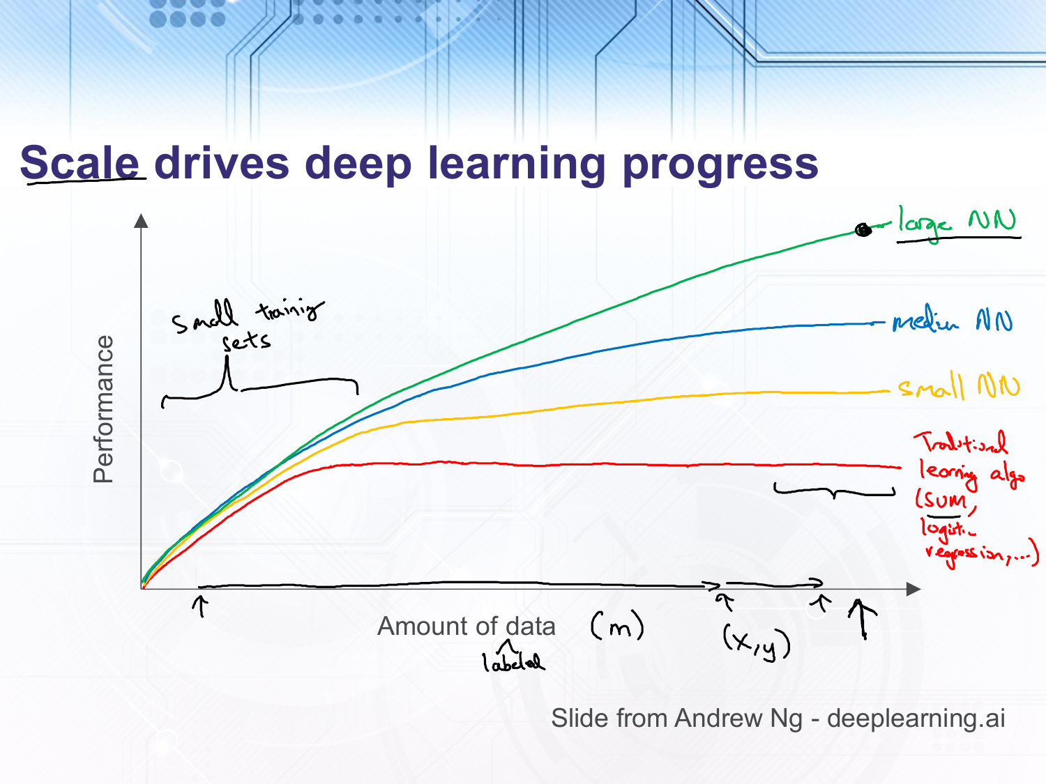
This slide is taken from an Andrew Ng course at deeplearning.ai. In it he argues that the reason deep learning has been increasingly successful is that we have more and more training data and more and more compute power. The traditional learning algorithms can do as well or even better than neural networks when the amount of training data is small. However, as the amount of training data increases their performance levels off whilst neural networks performance continues to increase. Additionally, the increase in computational power in conjunction with algorithmic breakthroughs which allow gradients to flow through large neural networks have meant that we can increase the size of our neural networks and gain increased performance.

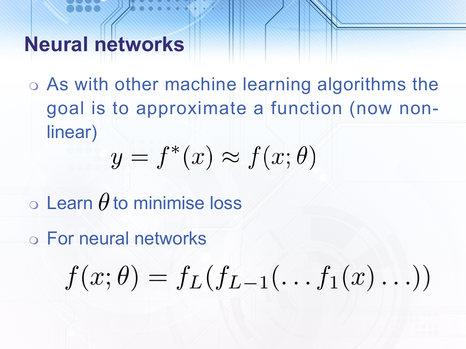
Neural networks, like other machine learning algorithms try to approximate a function, however the function is now non-linear. For neural networks it is in fact a chain of functions where each one is non-linear and each function is called a layer.

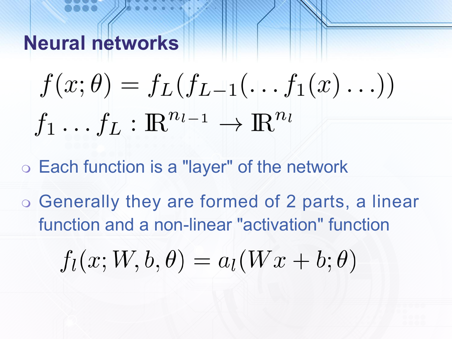
The input and output dimensions of the functions can vary. The form of the functions is generally to first apply a linear transformation and then a non-linear activation function.

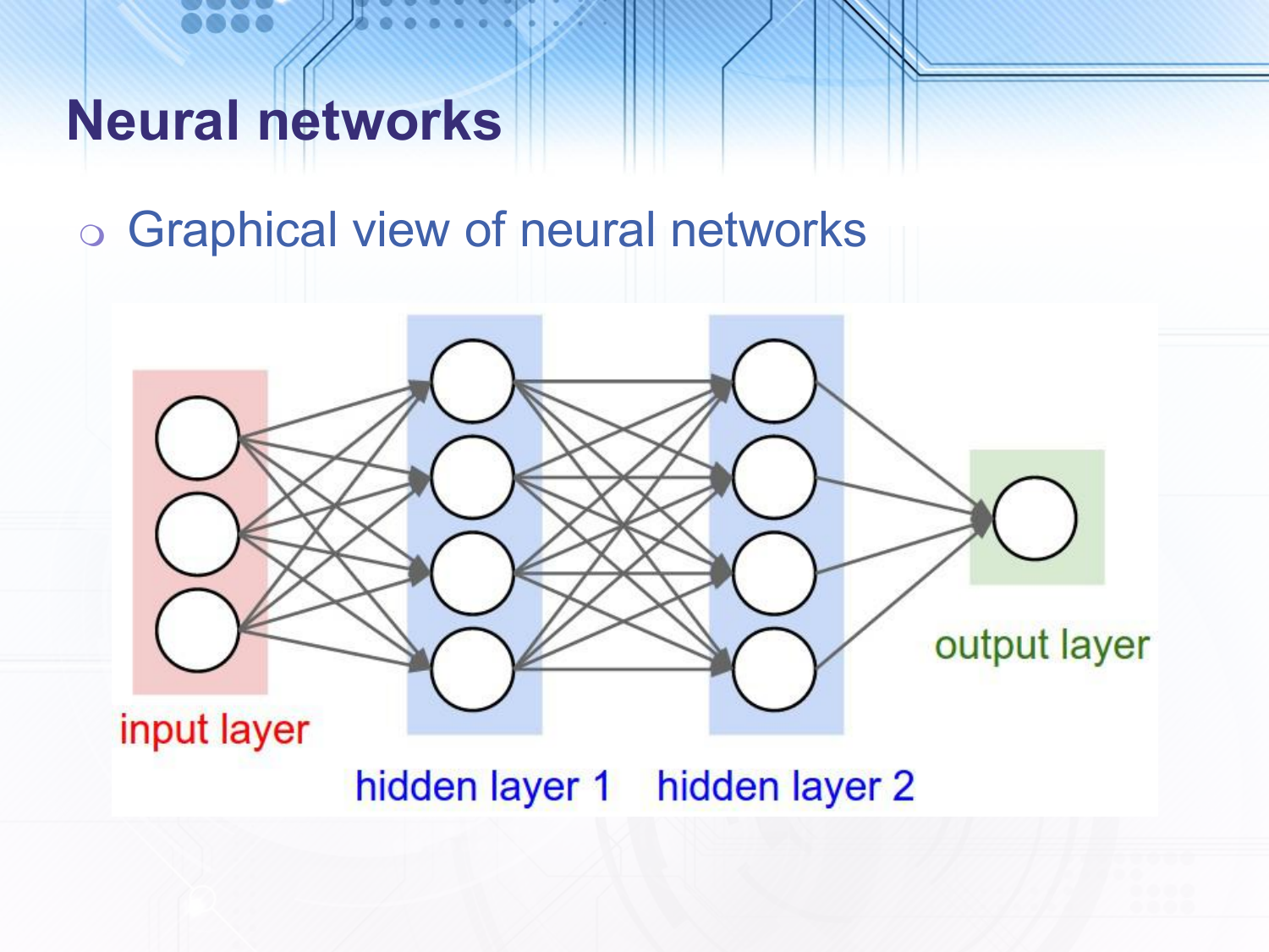
In the common graphical view of neural networks we represent each element of the vector passed to each layer as a node. In the above picture the we have three layers since the input layer has no function associated with it and is therefore not generally counted. The final layer in a neural network is called the output layer and all layers preceding it (not counting the input layer) are called hidden layers. In the above example all nodes in one layer are connected to all nodes in the following layer, this is called a fully connected neural network. Also, in this example all connections go forwards from the input layer to the output layer, this is called a feed-forward neural network.

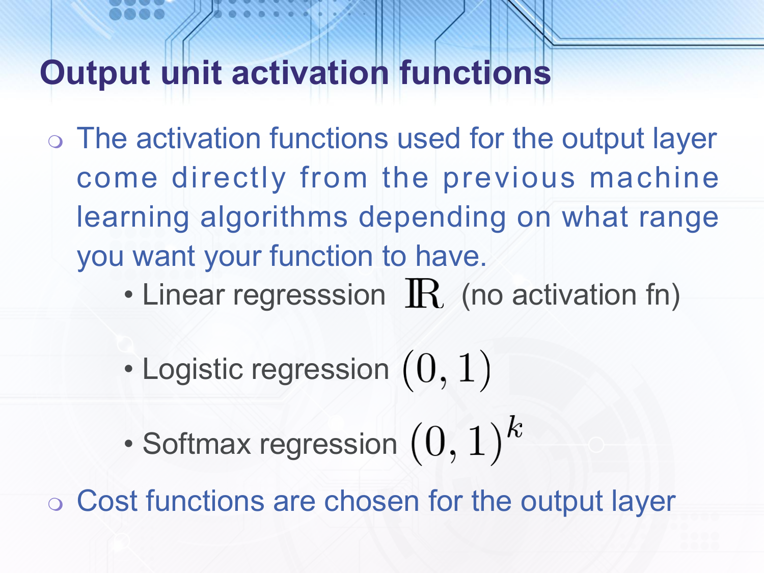
The output layer activation functions are chosen depending on what final form and what range you want your function to have, i.e. depending on whether you are doing regression or classification.

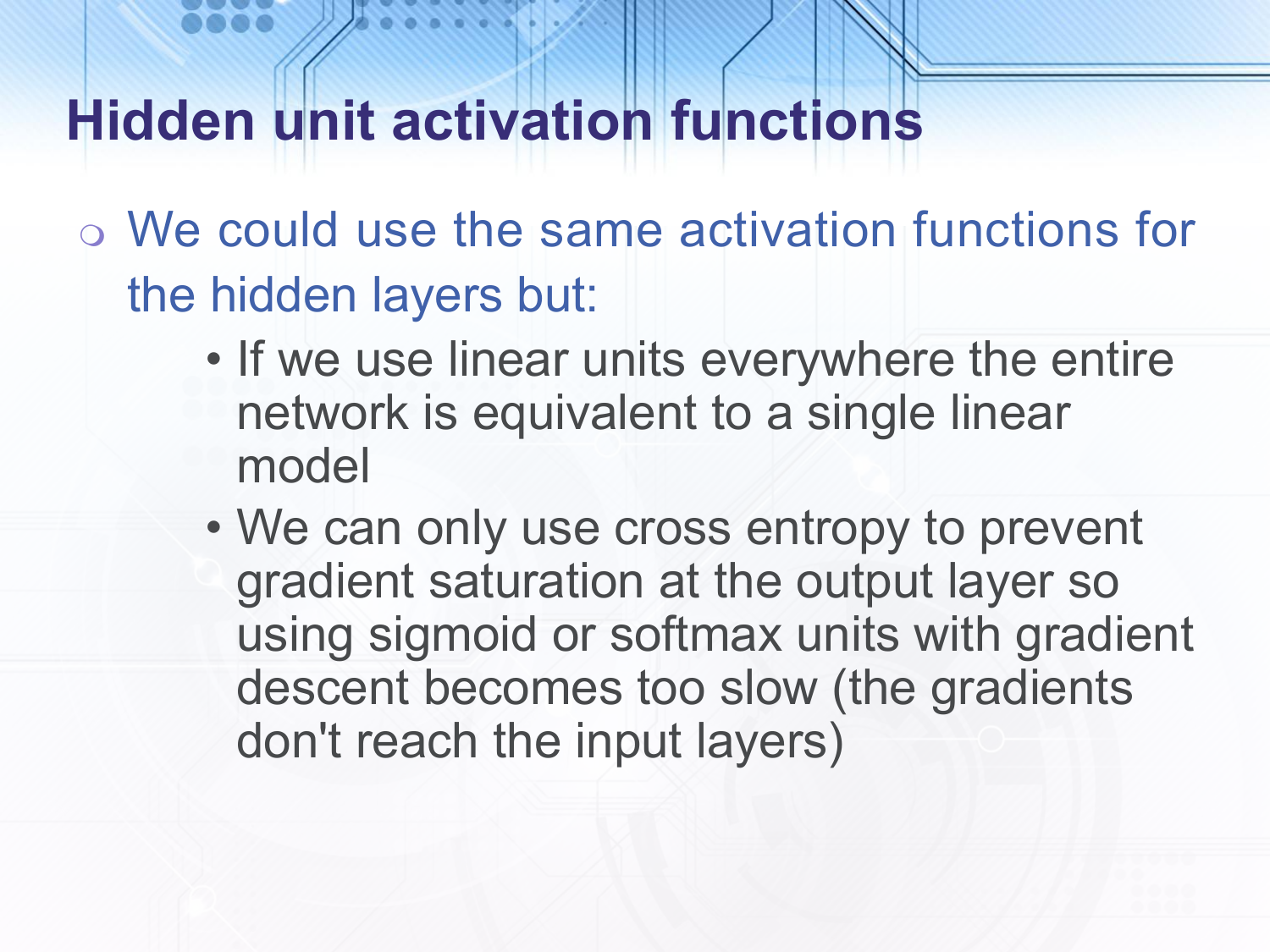
Previously, it has been common to use sigmoid (or tanh which is similar but $0$-centred) and linear functions in the hidden layers aswell, however this has some problems. Of course if all of the activation functions are linear then we do not add any non-linearity. Also, as mentioned in earlier slides the gradients of the sigmoid functions saturate even when the answer is incorrect, we only take the logarithm when applying the cost function at the output layer so hidden layers suffer from gradients being wiped out.

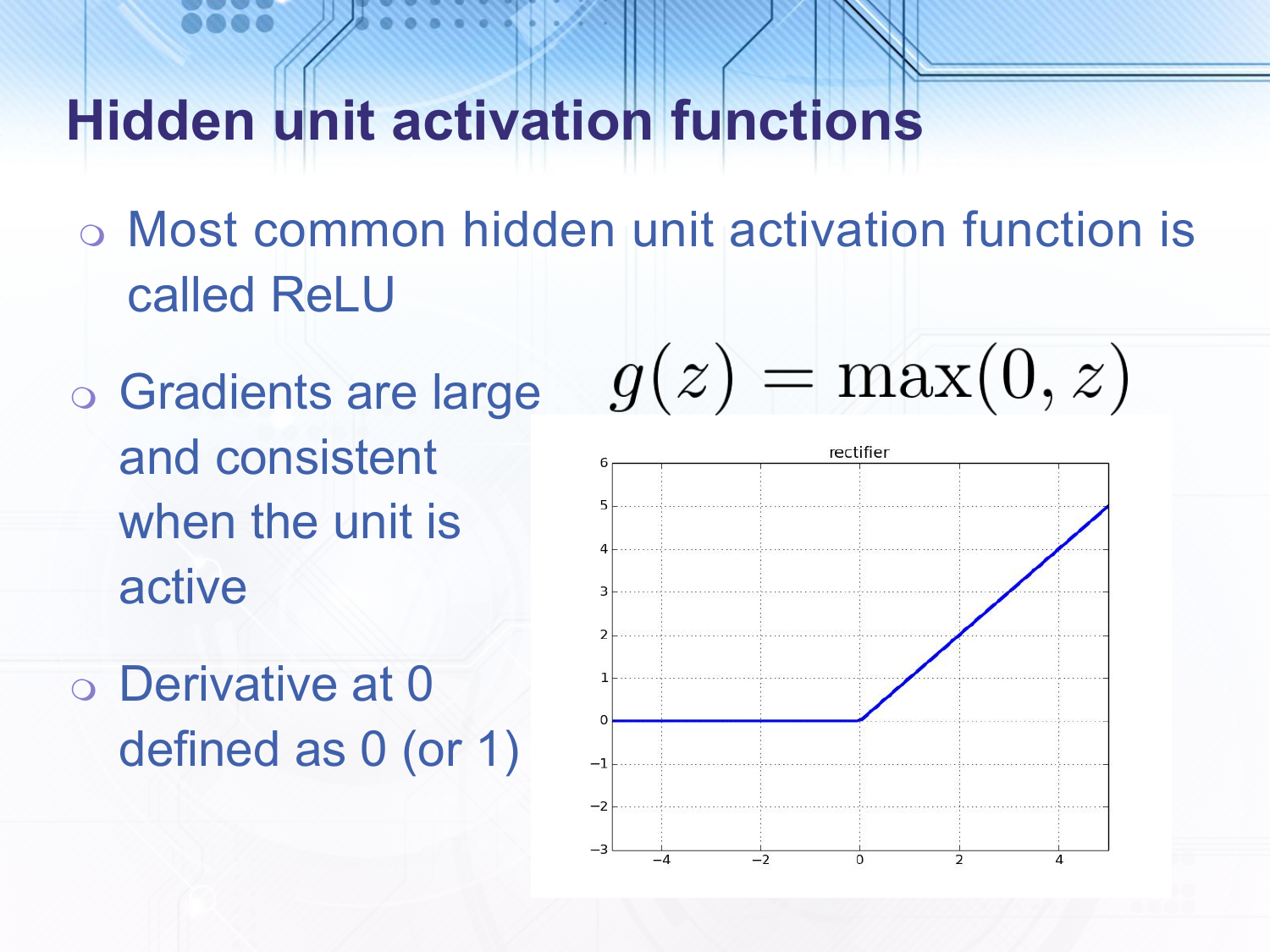
Instead, it is now more common to use a function called a ReLU, shown in the slide. This gives a large linear gradient for half of the input range so gradient saturation is less of a problem. One note is that although technically the gradient of the ReLU is undefined at $0$ if we simply treat it as though it is $0$ this does not cause problems.

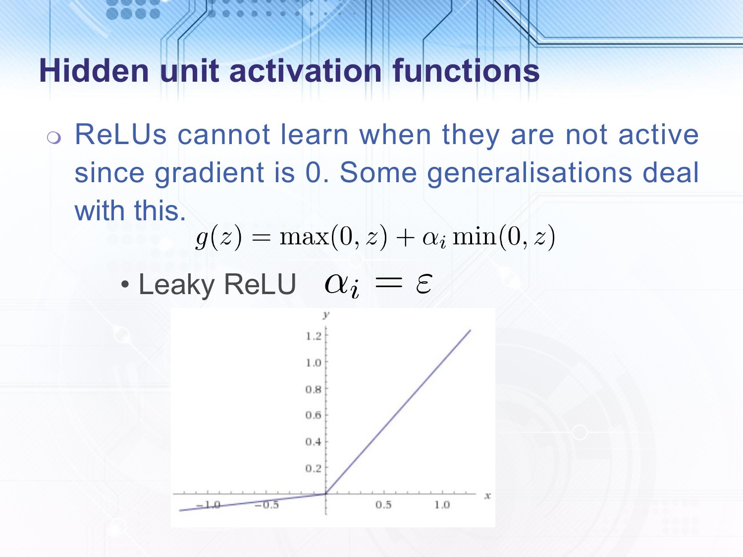
A similar activation function is called the leaky ReLU and does not entirely eliminate the gradient on the low input side.

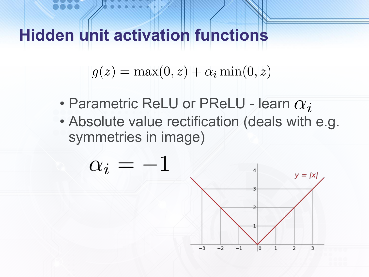
A parametric ReLU is similar to a leaky ReLU but allows the size of the gradient on the low input side to be learnt as a parameter rather than set to a single value. The absolute value rectifier is another variant where the low input side gives the same output as the high input side. This is only used in specific cases, e.g. to deal with symmetries in images.

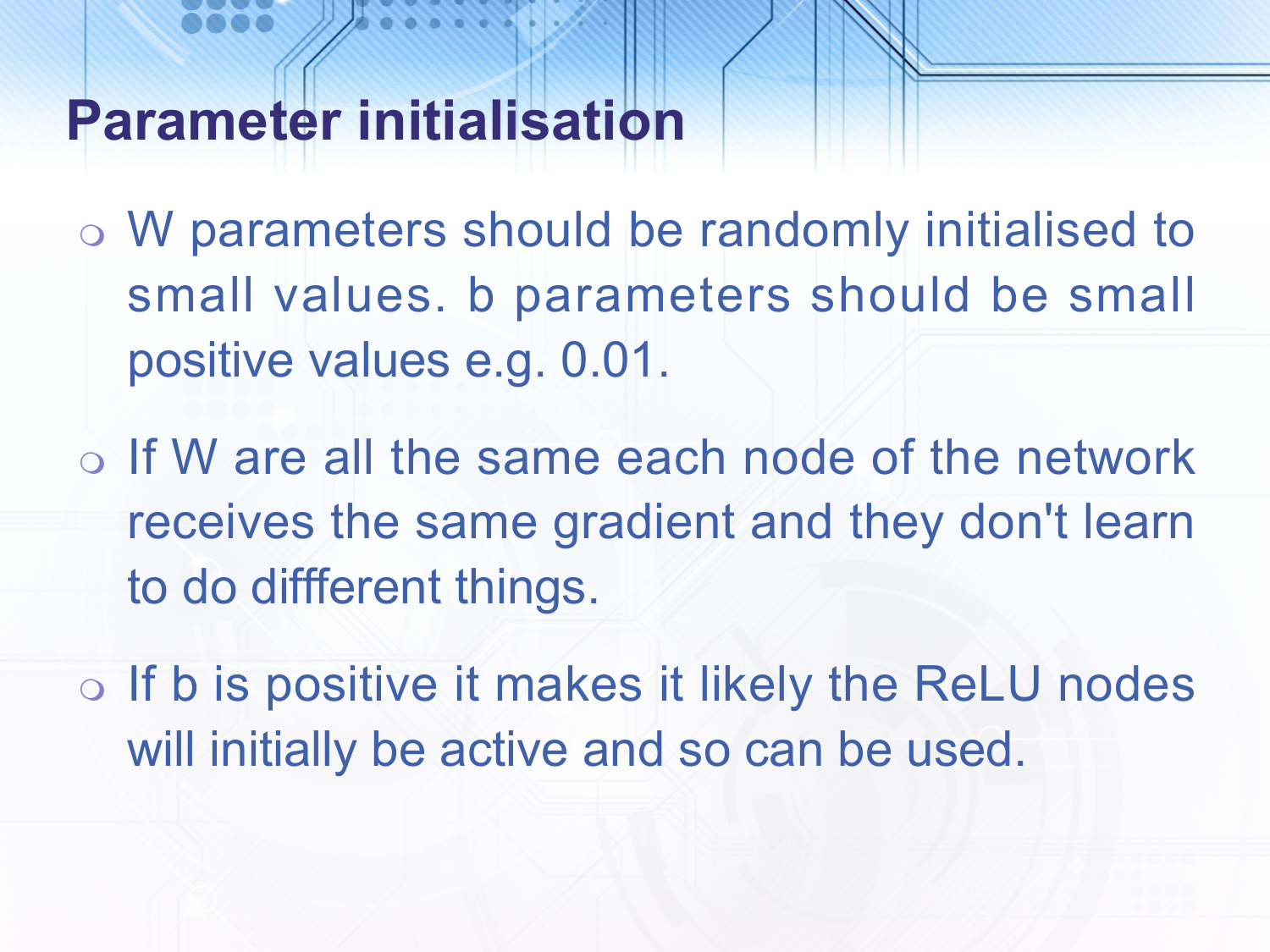
If all of the parameters are initialised to the same value e.g. 0 then each node receives the same gradient and they all update in exactly the same way, never breaking symmetries. Therefore they should be randomly initialised. In fact the size of the $W$ values should be set according to the size of the input, and possibly the size of the output. One common technique for this is called Xavier initialisation. However, I do not go into details of that here.

Forward propagation is the process of computing the output for a given input and a given set of parameters. To improve the parameters using, for example, gradient descent we must calculate the gradient of the cost function with respect to all of the parameters.

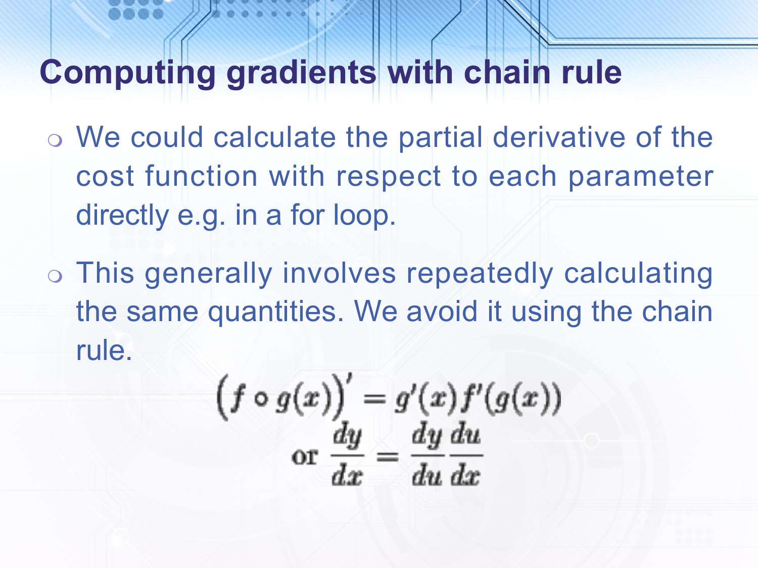
Doing this separately for each parameter would be highly inefficient because according to the chain rule the derivative of composed functions uses the derivative of the inner function i.e. the derivative of the cost function with respect to the parameters in the first hidden layer will use the derivative of the cost function with respect to the output of that layer. We apply the chain rule to determine expressions for the parameters in each layer and cache the intermediate results for reuse - this is called back propagation since we start by calculating derivatives for parameters in the final layer and then work our way backwards to the first hidden layer.

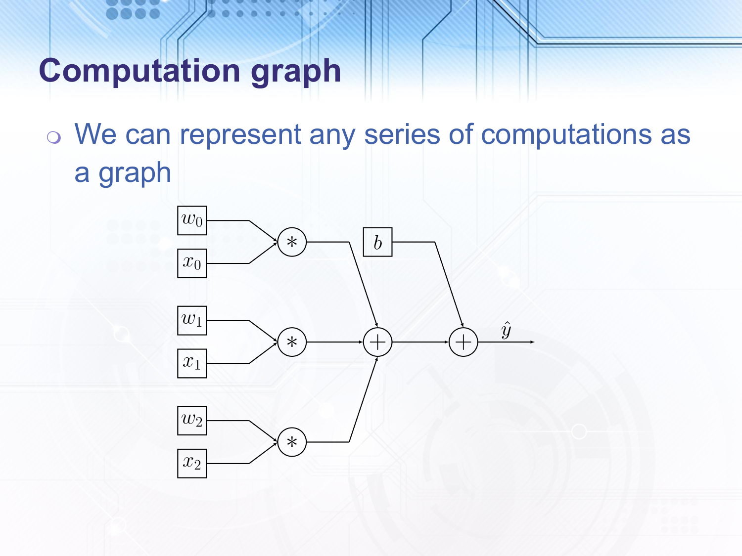
This can be easier to visualise using a graph. Any computation can be represented as a graph, for example this linear transformation. We can set up our computation graph at whatever level of detail we like as long as we can compute the gradient with respect to the input parameters and the tunable parameters. When this is used in real neural network applications we would typically have a linear transformation represented by one node instead of multiple as in this example.

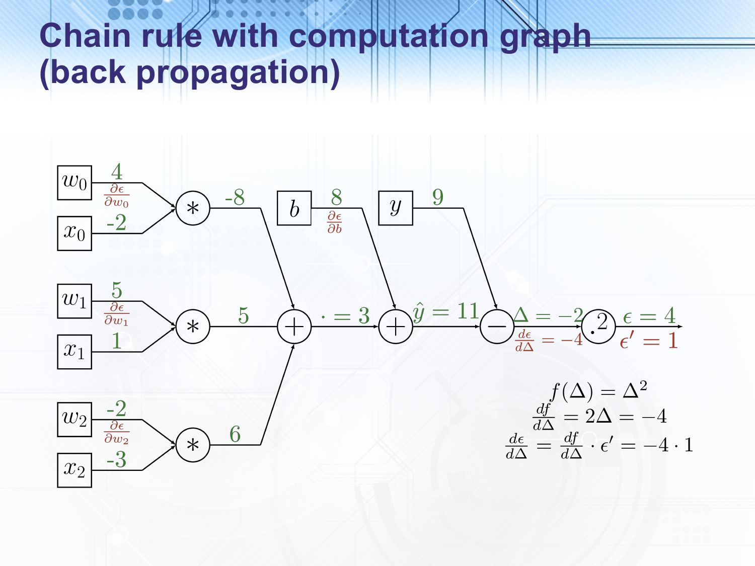
For example, given the inputs shown in green here calculated in the forward pass we can show how the gradient of the $\Delta$ variable is calculated. We start with a gradient of $1$ at the right hand side of the graph since the output of the final node is the full function and the gradient of the full function with respect to itself is always $1$. The last node represents squaring the input, so the derivative of the squaring function with respect to the input is $2 \Delta$. As the chain rule says we multiply the gradient of this function with respect to the input to this function by the gradient of the entire function with respect to the output to get $2 \cdot -2 \cdot 1 = -4$. This process continues through the other nodes.