CIFAR 10 Classification Using Softmax And Neural Networks
To gain experience in the practicalities of training machine learning algorithms I use the classic CIFAR 10 dataset for object recognition, which contains 60000 32x32 pixel colour images of 10 object categories. The dataset contains alot of challenging variation but we know that it is possible since human beings are capable of distinguishing the categories. The state of the art performance is around 95% using deep convolutional neural networks. I won’t achieve that level of performance as I will restrict myself to fully connected shallow networks, but this task will provide a good test bed for implementing some of the common algorithms used in deep learning and experimenting with tuning neural network parameters aswell as different regularisation and optimisation strategies.
import math
import numpy as np
import matplotlib.pyplot as plt
import accuracy_measures as am
from collections import namedtuple
from cifar10_web import cifar10
import copy
from functools import partial
from progress_bars import *
import random
from scipy.ndimage.interpolation import rotate
from scipy.ndimage.interpolation import shift

%matplotlib inline
One of the simplest classification methods is softmax classification, which is an extension of logistic regression to the multiclass problem and should converge to give the best linear split of the data.
We start by implementing the cost function, $J$ which calculates the cost of the fit for a set of data, $x$, and labels, $y$, given a set of parameters, $\theta$. It also returns the gradient vector:
In general let’s denote that we have $m$ data points (in our case images) and we use $i$ as the index to iterate over them, $n$ classes and we use $j$ as the index, and $p$ elements for each datapoint and use $k$ as the index. For softmax classification our hypothesis for a given data point being of each class is a vector where each element is the exponentiation of some linear transformation of the data point and the vector is then normalised to sum to 1. So the hypothesis for data point $i$ belonging to class $j$ is:
For the cost function we use the cross entropy:
where 1 is the indicator function i.e. it is 1 when $y_i=j$ and 0 otherwise.
The gradient of this with respect to the parameters $W, b$ can be calculated in terms of the gradient with respect to $z_{i,j}$:
Later we will address overfitting by adding a weight decay regularisation term to the cost function:
The gradient of the regularisation term is:
We can also calculate the gradient of the cost function with respect to the input, $x$, which will be useful later on.
Rather than storing $W$ and $b$ in our classifier directly we flatten them into a single $\theta$ vector, and reconstruct $W$ and $b$ from $\theta$ as required. This will make it easier to swap this classifier for other classifiers later. We can easily create functions to flatten and unflatten any number of arrays of any shapes as follows.
def get_flatten_weights_functions(*shapes):
    '''Return functions for flattening arrays of the shapes specified into a single vector,
    and reconstructing the arrays from a vector'''
    sizes = [np.prod(s) for s in shapes]
    # Taking the cumulative sum gives one past the end index for each array
    cumul_sizes = np.cumsum(sizes).reshape(len(sizes), 1)
    # Add the start index of each array
    cumul_start_end = np.hstack((np.vstack(([0], cumul_sizes[:-1])), cumul_sizes, shapes))

    def flatten_weights(*args):
        '''Flatten the arrays passed in to a single vector'''
        return np.hstack([a.flatten() for a in args]).reshape(cumul_sizes[-1, 0], 1)
    def unflatten_weights(theta):
        '''Reconstruct arrays from the single vector passed in'''
        return tuple(theta[c[0]:c[1]].reshape(c[2:]) for c in cumul_start_end)

    return flatten_weights, unflatten_weights
class Softmax:
    '''Softmax classifier'''

    def __init__(self, input_size, output_size, initialisation_method='zero'):
        '''Initialise the softmax parameters either to 0 or using Xavier initialisation,
        store parameters in theta vector and create functions for converting between
        the theta vector and the w and b parameters'''
        self.input_size = input_size
        w_shape = (input_size, output_size)
        b_shape = (1, output_size)
        if initialisation_method == 'zero':
            w = np.zeros(w_shape)
            b = np.zeros(b_shape)
        elif initialisation_method == 'random':
            # Our random initialisation is a common simplification of Xavier initialisation
            # (Understanding the difficulty of training deep feedforward neural networks -
            # Glorot & Bengio) which is used for example by the Caffe framework
            w = (1.0/input_size) * np.random.normal(size=w_shape)
            b = np.zeros(b_shape)

        # Store all theta parameters in a 1d vector to allow use with generic
        # optimisation algorithms
        # For convenience store functions to flatten w, b into theta and to vice versa
        self.flat, self.unflat = get_flatten_weights_functions(w_shape, b_shape)
        self.theta = self.flat(w, b)

    def hypothesis_with_unpacked_w(self, x):
        '''
        Return the hypothesis h for each data point in x and the unpacked w for
        convenience
        '''
        w, b = self.unflat(self.theta)
        # z is the linear transformation of input x, to which we apply the softmax
        z = x @ w + b
        exp_output = np.exp(z)
        exp_sum = np.sum(exp_output, axis=1).reshape(exp_output.shape[0],1)
        h = np.divide(exp_output, exp_sum)
        return h, w

    def hypothesis(self, x):
        '''
        Return the hypothesis h for each data point in x
        '''
        h, w = self.hypothesis_with_unpacked_w(x)
        return h

    def cost_function_with_h_w(self, x, y, reg):
        '''
        Return the cost function used for softmax regression for the given values of
        x, y and the regularisation strength. Also return the hypothesis h for each
        data point in x and the unpacked w for convenience
        '''
        h, w = self.hypothesis_with_unpacked_w(x)
        # Cost per example is log of hypothesis for actual y
        cost_per_training_example = -np.log(h[np.arange(len(x)), y])
        # Overall cost is average cost per example + regularisation strength *
        # weight decay cost i.e. sum of w parameters squared
        m = cost_per_training_example.shape[0]
        cost = (1/m)*np.sum(cost_per_training_example) + (reg/2)*np.sum(w**2)
        return cost, h, w

    def cost_function(self, x, y, reg):
        '''
        Return the cost function used for softmax regression for the given values of
        x, y and the regularisation strength
        '''
        cost, h, w = self.cost_function_with_h_w(x, y, reg)
        return cost

    def cost_function_with_z_grad(self, x, y, reg):
        '''
        Return the cost function used for softmax regression and its derivative with
        respect to the parameters w and b (flattened to theta vector) and with respect to
        z - the linear transformation wx + b for the given values of x, y and the
        regularisation strength. Also return w for convenience.
        '''
        cost, h, w = self.cost_function_with_h_w(x, y, reg)
        grad_wrt_z = h
        m = x.shape[0]
        grad_wrt_z[np.arange(m), y] -= 1
        grad_wrt_z /= m

        grad = self.flat(x.T @ grad_wrt_z + reg*w, np.sum(grad_wrt_z, axis=0))
        return cost, grad, grad_wrt_z, w

    def cost_function_with_x_grad(self, x, y, reg):
        '''
        Return the cost function used for softmax regression and its derivative with
        respect to the parameters w and b (flattened to theta vector) and with respect to
        the input x for the given values of x, y and the regularisation strength
        '''
        cost, grad, grad_wrt_z, w = self.cost_function_with_z_grad(x, y, reg)
        dx = grad_wrt_z @ w.T
        return cost, grad, dx

    def cost_function_with_grad(self, x, y, reg):
        '''
        Return the cost function used for softmax regression and its derivative with
        respect to the parameters w and b (flattened to theta vector) for the given values
        of x, y and the regularisation strength
        '''
        cost, grad, grad_wrt_z, w = self.cost_function_with_z_grad(x, y, reg)
        return cost, grad
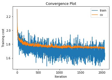
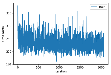
We can now train and test softmax regression on our data. We use mini-batch gradient descent with learning rate decay. To help tune the hyper-parameters we output the training and cross validation costs per iteration and the size of the gradient squared.
There are a few things to note about our gradient descent implementation:
- We have the option to alter the data before adding it to the training batch. This will allow us to synthesize additional data for example by translating or rotating images.
- We have implemented a numerical check on the gradient which we can turn on to test whether our analytical gradient calculation is implemented correctly.
- The algorithm uses early stopping i.e. we evaluate the cross validation cost for our classifier parameters as we run the algorithm and keep track of the parameters which give the best result. This is a form of regularisation which is in some problems equivalent to using weight decay in the cost function.
def run_gradient_descent(classifier, x, y, reg, x_cv, y_cv, num_iterations=1000,
                         learning_rate=0.001, learning_rate_decay=0.99, batch_size=200,
                         progress_fun=None, numerical_gradient_check_eps=None,
                         alter_data_point=None, max_iterations_without_improvement=None):
    '''
    Run mini batch gradient descent on the parameters of the classifier passed in.
    The parameters must be stored as an array called theta.

    The classifier must have functions:
    - cost_function - taking input x, labels y and regularisation strength and returning a
    scalar
    - cost_function_with_grad - as cost_function but also returning gradient with respect to
    theta
    The classifier may optionally have a function:
    - cost_function_with_x_grad - as cost_function_with_grad but also returning gradient
    with respect to the input x

    Apart from the classifier the caller must pass in:
    x - input training data
    y - training data labels
    reg - regularisation strength
    x_cv - input cross validation data
    y_cv - cross validation labels
    num_iterations - number of gradient descent steps to take
    learning_rate - factor to multiply negative gradient by when taking a step
    learning_rate_decay - factor to multiply learning rate by after each epoch
    batch_size - number of data points per mini batch
    progress_fun - if not None a function which will be called with progress through iterations
    numerical_gradient_check_eps - if not None we will perform a numerical gradient check on
    classifier functions returning gradients using the value passed as our epsilon
    alter_data_point - if not None we will apply this function to each data point before adding
    it to a mini batch
    max_iterations_without_improvement - if we get this many iterations without the cross
    validation score improving then we have converged so stop training
    '''

    # Randomly permute the data before we start in case there is any grouping
    costs = np.zeros((num_iterations, 1))
    costs_cv = np.zeros((num_iterations, 1))
    grad_norm = np.zeros((num_iterations, 1))
    num_iterations_per_epoch = math.ceil(x.shape[0] / batch_size)

    best_cost_cv = 1e9
    best_iteration = 0
    for iteration in range(num_iterations):
        randIndices = np.random.choice(range(x.shape[0]), (batch_size,), replace=True)
        x_batch = x[randIndices,:]
        y_batch = y[randIndices]

        if alter_data_point is not None:
            for data_index in range(batch_size):
                x_batch[data_index] = alter_data_point(x_batch[data_index])

        cost, grad = classifier.cost_function_with_grad(x_batch, y_batch, reg)
        cost_cv = classifier.cost_function(x_cv, y_cv, reg)

        # If we want to check that we have implemented the gradient correctly we can approximate
        # it numerically and see if it is close enough to the analytical gradient we calculated
        if numerical_gradient_check_eps is not None:
            original_theta = copy.deepcopy(classifier.theta)
            gradCosts = np.zeros(original_theta.shape)
            for i in range(len(original_theta)):
                classifier.theta = copy.deepcopy(original_theta)
                classifier.theta[i] += numerical_gradient_check_eps
                gradCosts[i] = classifier.cost_function(x_batch, y_batch, reg)
                grad_estimate = (gradCosts[i] - cost)/numerical_gradient_check_eps
                assert (np.abs(grad[i] - grad_estimate) < 100*numerical_gradient_check_eps),\
                    "numerical grad estimate is {0} analytical grad is {1}".format(grad_estimate, grad[i])
            grad_estimate = (gradCosts - cost)/numerical_gradient_check_eps
            print(np.amax(np.abs(grad-grad_estimate)))
            assert np.all(np.abs(grad-grad_estimate) < 100*numerical_gradient_check_eps)
            classifier.theta = copy.deepcopy(original_theta)

            if hasattr(classifier, 'cost_function_with_x_grad'):
                original_x = copy.deepcopy(x_batch)
                cost, grad, grad_wrt_x = classifier.cost_function_with_x_grad(original_x, y_batch, reg)
                grad_estimates = np.zeros(grad_wrt_x.shape)
                for i in range(grad_wrt_x.shape[0]):
                    for j in range(grad_wrt_x.shape[1]):
                        current_x = copy.deepcopy(original_x)
                        current_x[i, j] += numerical_gradient_check_eps
                        diff = current_x - original_x
                        gradCost = classifier.cost_function(current_x, current_y, reg)
                        grad_estimates[i, j] = (gradCost - cost)/diff[i,j]
                        assert (np.abs(grad_wrt_x[i, j] - grad_estimates[i, j]) < 100*numerical_gradient_check_eps),\
                            "numerical grad estimate is {0} analytical grad is {1}".format(grad_estimates[i, j], grad_wrt_x[i, j])
                print(np.amax(np.abs(grad_wrt_x-grad_estimates)))
                assert np.all(np.abs(grad_wrt_x-grad_estimates) < 100*numerical_gradient_check_eps)

        classifier.theta -= learning_rate*grad

        if cost_cv < best_cost_cv:
            best_cost_cv = cost_cv
            best_theta = classifier.theta
            best_iteration = iteration
        costs[iteration, 0] = cost
        costs_cv[iteration, 0] = cost_cv
        # Return the grad norm so that we can see if we have reached a local minimum
        grad_norm[iteration, 0] = np.sqrt(np.sum(grad**2))

        if iteration % num_iterations_per_epoch == 0:
            learning_rate *= learning_rate_decay

        if progress_fun is not None:
            progress_fun((iteration+1)/num_iterations)

        # If we haven't made any progress for a lot of iterations assume we have converged
        if max_iterations_without_improvement is not None and
          iteration > best_iteration + max_iterations_without_improvement:
            break

    # use the parameters which give the lowest cv cost
    classifier.theta = best_theta

    return costs.flatten(), grad_norm.flatten(), costs_cv.flatten()
Statistics = namedtuple('Statistics', ['costs', 'grad_norm', 'costs_cv'])

def train_and_test_prob_estimator(
    classifier, x_train, y_train, x_cv, y_cv, reg, **grad_descent_kwargs):
    '''Run gradient descent and calculate the predicted labels and the cost for the
    training data and cross validation data aswell as statistics from the gradient
    descent algorithm'''

    # Do a numerical optimisation to minimise the cost function on the training dataset
    # then return the parameters theta so we can evaluate the hypothesis on the test dataset
    costs, grad_norm, costs_cv = run_gradient_descent(
        classifier, x_train, y_train, reg, x_cv, y_cv, **grad_descent_kwargs)

    cost_train = classifier.cost_function(x_train, y_train, reg)
    h_train = classifier.hypothesis(x_train)
    cost_cv = classifier.cost_function(x_cv, y_cv, reg)
    h_cv = classifier.hypothesis(x_cv)

    y_train_predicted = np.argmax(h_train, axis=1)
    y_cv_predicted = np.argmax(h_cv, axis=1)

    statistics = Statistics(costs=costs, costs_cv=costs_cv, grad_norm=grad_norm)

    return y_train_predicted, cost_train, y_cv_predicted, cost_cv, statistics

def train_and_test_softmax_regression_gradient_descent(
    x_train, y_train, x_cv, y_cv, reg, num_classes, **prob_estimator_kwargs):
    '''Create a softmax classifier, run gradient descent and calculate the predicted labels
    and the cost for the training data and cross validation data aswell as statistics
    from the gradient descent algorithm'''

    sm = Softmax(x_train.shape[1], num_classes)
    y_train_predicted, cost_train, y_cv_predicted, cost_cv, statistics = train_and_test_prob_estimator(
        sm, x_train, y_train, x_cv, y_cv, reg, **prob_estimator_kwargs)

    return y_train_predicted, cost_train, y_cv_predicted, cost_cv, statistics
def plot_statistics(statistics):
    '''Plot the training and cross validation costs and the squared gradient over the
    course of the gradient descent algorithm'''
    plt.figure()
    plt.plot(statistics.costs, label='train')
    plt.plot(statistics.costs_cv, label='cv')
    plt.xlabel('Iteration')
    plt.ylabel('Training cost')
    plt.title('Convergence Plot')
    plt.legend()
    plt.show()

    plt.figure()
    plt.plot(statistics.grad_norm, label='train')
    plt.xlabel('Iteration')
    plt.ylabel('Grad Norm')
    plt.legend()
    plt.show()
Lets read in our data and see how softmax regression does. We split the training data into a training set and cross validation set. The test set is separate and will be used later. We compute the mean image from the training data and subtract it from each image so that we have 0 centred data.
def read_data():
    '''Read the CIFAR data, split it into training, cross validation and test, and 0
    centre it'''
    train_images, train_labels, test_images, test_labels = cifar10(path='/home/michael/python-cifar')
    train_images *= 255
    test_images *= 255
    train_images = train_images.reshape(train_images.shape[0], 3, 32, 32).transpose(0, 2, 3, 1).reshape(train_images.shape[0], 3*32*32)
    test_images = test_images.reshape(test_images.shape[0], 3, 32, 32).transpose(0, 2, 3, 1).reshape(test_images.shape[0], 3*32*32)
    cv_proportion = 0.02
    num_cv = int(train_labels.shape[0]*cv_proportion)
    num_train = train_labels.shape[0] - num_cv
    train_images, cv_images = np.vsplit(train_images, [num_train])
    train_labels, cv_labels = np.vsplit(train_labels, [num_train])

    mean_image = np.mean(train_images, axis=0)
    train_images -= mean_image
    cv_images -= mean_image
    test_images -= mean_image

    return train_images, np.argmax(train_labels, axis=1), cv_images, np.argmax(cv_labels, axis=1), test_images, np.argmax(test_labels, axis=1)

x_train, y_train, x_cv, y_cv, x_test, y_test = read_data()
def reshape_to_image(data):
    return data.reshape(32, 32, 3)
plt.figure()
im = copy.deepcopy(reshape_to_image(x_train[0,:]))
im -= im.min()
im *= 1.0/im.max()
plt.imshow(im)

Although we don’t have too many hyperparameters in the softmax classifier it can become difficult to find combinations which work, for example choosing the best learning rate and regularisation strength. One option is to create a grid of hyperparameter combinations where we use the same learning rate with a number of different regularisation stengths. With this strategy, if we have time to run gradient descent 25 times we could for example use 5 learning rates and 5 regularisation strengths. However, in some cases one hyperparameter will have a much bigger influence on the cost we reach than another so getting it exactly right is important. Therefore it is usually more useful to sample points at random from the joint hyperparameter space. This way we get 25 different values for the important hyperparameter which should give a clear view of how it affects the cost, whilst the costs for the less important hyperparameter will be dominated by the more important one. This way we can efficiently set the most important hyperparameters first.
def select_log_space_point(start, end, base, return_shape):
    '''Select a point which is uniformly distributed in logarithmic space between start
    and end'''
    minb = min([1, base])
    maxb = max([1, base])
    return start + (base**np.random.rand(*return_shape) - minb)*((end - start)/(maxb - minb))
def get_hyperparameter_combinations(num_points_to_sample=10, **kwargs):
    '''For each parameter passed in kwargs, if it is a list of 2 numbers select
    num_points_to_sample values between these numbers randomly in log space, if it is a
    single number repeat it num_points_to_sample times'''
    kwarg_sets = []
    for hp_name, hp in kwargs.items():
        if type(hp) is list:
            if len(hp) == 2:
                # If we get a range select points within it in log space
                kwargs[hp_name] = select_log_space_point(hp[0], hp[1], 10, (num_points_to_sample,))
            else:
                assert len(hp) == num_points_to_sample
                kwargs[hp_name] = np.array(hp)
        else:
            kwargs[hp_name] = np.full((num_points_to_sample,), hp)

    return [{hp_name : hp[i] for hp_name, hp in kwargs.items()} for i in range(num_points_to_sample)]
def plot_hyperparameter_combos(optimisation_routine, x_train, y_train, x_cv, y_cv,
                               num_classes, **kwargs):
    '''For any kwargs which start hp_ remove these characters and pass them into
    get_hyperparameter_combinations to sample points between the range specified.
    hp_num_points_to_sample should also be passed in.
    Run the optimisation_routine passed in on the data passed in with the kwargs and each
    sample of hp parameters. Then plot graphs for the hp parameters against cost.
    '''
    hp_kwargs = {k[3:]: v for k, v in kwargs.items() if k.find('hp_') == 0}
    hp_combos = get_hyperparameter_combinations(**hp_kwargs)
    kwargs = {k: v for k, v in kwargs.items() if k.find('hp_') != 0}

    y_train_predicted_all = []
    cost_train_all = []
    y_cv_predicted_all = []
    cost_cv_all = []
    statistics_all = []

    # We pass reg in as a normal arg not a keyword arg, it could be in either
    # hps or kwargs so get it out of whichever one contains it.
    reg = None
    if 'reg' in kwargs:
        reg = kwargs['reg']
        del kwargs['reg']

    if 'progress_fun' in kwargs:
        passed_progress_fun = copy.copy(kwargs['progress_fun'])

    for i, hps in enumerate(hp_combos):
        if 'progress_fun' in kwargs:
            kwargs['progress_fun'] = partial(multi_stage_progress, i, len(hp_combos),
                                             passed_progress_fun)

        if 'reg' in hps:
            hp_kwargs = copy.deepcopy(hps)
            del hp_kwargs['reg']
            reg = hps['reg']
        else:
            hp_kwargs = hps

        y_train_predicted, cost_train, y_cv_predicted, cost_cv, statistics = \
        optimisation_routine(x_train, y_train, x_cv, y_cv, reg, num_classes,
                             **kwargs, **hp_kwargs)

        y_train_predicted_all.append(y_train_predicted)
        cost_train_all.append(cost_train)
        y_cv_predicted_all.append(y_cv_predicted)
        cost_cv_all.append(cost_cv)
        statistics_all.append(statistics)

    for k in hp_combos[0].keys():
        plt.figure()
        plt.title(k)
        sorted_lr, sorted_cost_train = zip(*sorted(zip([hps[k] for hps in hp_combos], [np.mean(s.costs[-5:]) for s in statistics_all])))
        plt.plot(np.array(sorted_lr), np.array(sorted_cost_train))

    return y_train_predicted_all, cost_train_all, y_cv_predicted_all, cost_cv_all, statistics_all
We’ll try 10 samples for 300 iterations each with different learning rates and regularisation strengths.
y_train_predicted_all, cost_train_all, y_cv_predicted_all, cost_cv_all, statistics_all = \
plot_hyperparameter_combos(train_and_test_softmax_regression_gradient_descent,
                           x_train, y_train, x_cv, y_cv, 10,
                           num_iterations=300, progress_fun=create_progress_bars_and_get_update_fun(),
                           hp_num_points_to_sample=10, hp_learning_rate=[1e-7, 1e-5],
                           learning_rate_decay=0.95, hp_reg=[0.0, 0.3])
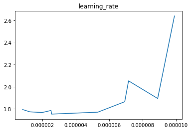
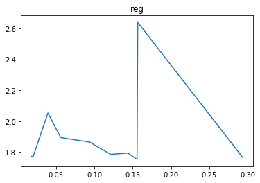
In this case we can see that the learning rate parameter has a clear effect on the cost with around 3e-6 giving the best result whilst the regularisation strength has little effect. Therefore, for now we’ll leave the regularisation strength at 0 and try extra iterations with our found learning rate.
y_train_predicted, cost_train, y_cv_predicted, cost_cv, statistics = \
    train_and_test_softmax_regression_gradient_descent(x_train, y_train, x_cv, y_cv, 0.00, 10,
                                                       learning_rate=3e-6, learning_rate_decay=0.95,
                                                       num_iterations=10000, max_iterations_without_improvement=500,
                                                       progress_fun=create_progress_bars_and_get_update_fun())

plot_statistics(statistics)

am.print_multiclass_accuracy_measures(y_train_predicted, y_train, cost_train, 'training')
am.print_multiclass_accuracy_measures(y_cv_predicted, y_cv, cost_cv, 'cv')
training  cost  1.67865964494 , accuracy  0.428326530612
cv  cost  1.75438101211 , accuracy  0.403
The training and cross validation costs initially decrease quickly and then much slower indicating that we have probably set our learning rate well. Also the squared gradient norm decreases to a low value and remains low which indicates that we are close to a local minimum. In the softmax regression case for each mini batch of data we have a convex cost function so for each mini batch the local minimum must also be the global minimum. Of course these minimums may not be co-located with the minimum of the cost function on all of the data but it is common to assume that they are nearby.
The accuracy on the training data reaches 42.8% whilst the accuracy on the cross validation data reaches 40.3%. It is normal for the performance on the cross validation set to be lower than that on the training data set since the model is being fitted directly to the training data set. In this case the difference is small which indicates that we have not overfitted to the training data. Since the accuracy achieved is low either the input data is not sufficiently informative to distinguish the classes or the model does not have the capacity to represent the function we are trying to approximate. In this case we know that the input data is sufficiently informative to achieve classification accuracy of 95% since that is the state of the art, therefore our model is too low capacity.
One way to see how much the model is overfitting or underfitting is to plot how the training costs and cross validation costs change as we increase the amount of data we allow for training. This is sometimes called the learning curve.
def plot_learning_curve(x_train, y_train, x_cv, y_cv, reg, optimisation_routine,
                        min_data=5, max_data=None, num_points=20,
                        plot_convergence_for_each_point=False, **optimisation_kwargs):
    '''Run the optimisation routine passed in with the data passed in restricting the
    amount of training data used to different amounts starting with min_data and then
    increasing in log space to max_data or the number of training examples available
    if max_data is not specified so that there are num_points in total. If
    plot_convergence_for_each_point is set to True then plot graphs showing how each
    point converges. Other kwargs will be passed to the optimisation routine'''
    if max_data is None:
        max_data = x_train.shape[0]

    num_to_train_list = np.round(np.geomspace(min_data, max_data, num=num_points, dtype=np.float32)).\
        astype(np.uint32)

    # If we are keeping track of our progress in the optimisation routine deal with the fact we are
    # running the optimsation routine multiple times
    if 'progress_fun' in optimisation_kwargs:
        passed_progress_fun = copy.copy(optimisation_kwargs['progress_fun'])

    costs_train = np.zeros((num_points, 1))
    costs_cv = np.zeros((num_points, 1))
    for i in range(len(num_to_train_list)):
        num_to_train = num_to_train_list[i]

        if 'progress_fun' in optimisation_kwargs:
            optimisation_kwargs['progress_fun'] = partial(multi_stage_progress, i, len(num_to_train_list),
                                                          passed_progress_fun)

        y_train_predicted, costs_train[i], y_cv_predicted, costs_cv[i], statistics = \
        optimisation_routine(x_train[:num_to_train, :], y_train[:num_to_train],
                             x_cv, y_cv, 0.03, 10, **optimisation_kwargs)

        if plot_convergence_for_each_point:
            plot_statistics(statistics)

    am.print_multiclass_accuracy_measures(y_train_predicted, y_train[:num_to_train],
                                          costs_train[-1], 'training')
    am.print_multiclass_accuracy_measures(y_cv_predicted, y_cv, costs_cv[-1], 'cv')

    plt.figure()
    plt.plot(num_to_train_list, costs_train, label='$J_{\mathrm{train}}$')
    plt.plot(num_to_train_list, costs_cv, label='$J_{\mathrm{cv}}$')
    plt.xlabel('Num data points')
    plt.ylabel('Cost')
    plt.legend()
    plt.show()
plot_learning_curve(x_train, y_train, x_cv, y_cv, 0.00,
                    train_and_test_softmax_regression_gradient_descent,
                    learning_rate=3e-6, learning_rate_decay=0.95, num_iterations=300,
                    progress_fun=create_progress_bars_and_get_update_fun())
training  cost  [ 1.73935463] , accuracy  0.409102040816
cv  cost  [ 1.7786507] , accuracy  0.411
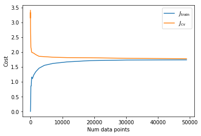
As expected we need a higher capacity model to describe the variation in classes. One way of doing this is to turn our model into a neural network by adding additional layers which do a linear transformation followed by a non-linear squashing function, in this case we will use ReLUs as our squashing function. Although for images it is better to use convolutional architectures which would allow deeper models, for simplicity I will just use a few fully connected layers.
class ReluLayer:
    '''ReLU layer - provides hypothesis and cost function for a layer which applies
    a linear transformation and then a ReLU to the input then passes this to an
    output layer'''

    def __init__(self, input_size, hidden_size, output_layer,
                 dropout_prob=None):
        '''Initialise the ReLU layer parameters using Xavier initialisation,
        store parameters in theta vector and create functions for converting between
        the theta vector and the w and b parameters'''

        self.dropout_prob = dropout_prob
        self.output_layer = output_layer

        w_shape = (input_size, hidden_size)
        b_shape = (1, hidden_size)

        # Our random initialisation is from the scheme described
        # https://arxiv.org/abs/1502.01852 which specialises Xavier initialisation
        # for ReLU
        w = 2.0/input_size * np.random.normal(size=w_shape)
        b = np.zeros(b_shape)

        # Store all theta parameters in a 1d vector to allow use with generic optimisation algorithms
        # For convenience store functions to flatten w, b into theta and to vice versa
        self.flat, self.unflat = get_flatten_weights_functions(w_shape, b_shape, output_layer.theta.shape)
        self.theta = self.flat(w, b, output_layer.theta)

    def hidden_layer_output(self, x):
        '''
        Return the result of applying the linear transformation and the ReLU to each data
        point in x, also return the unpacked w for convenience
        If the dropout_prob is not None apply the dropout algorithm aswell
        '''
        w, b, theta_upstream = self.unflat(self.theta)
        self.output_layer.theta = theta_upstream

        # Hidden layer
        l = x @ w + b
        hidden = np.maximum(0, l)
        if self.dropout_prob is not None:
            dropout_mask = (np.random.rand(*hidden.shape) < self.dropout_prob) / self.dropout_prob
            hidden *= dropout_mask
        return hidden, w

    def hypothesis(self, x):
        '''
        Return the hypothesis h for each data point in x
        '''
        # Compute the forward pass
        hidden, w = self.hidden_layer_output(x)

        # Output layer - Apply softmax regression
        return self.output_layer.hypothesis(hidden)

    def cost_function_with_w(self, x, y, reg):
        '''
        Return the cost function for the given values of x, y and the regularisation
        strength by passing this layer's output to the output layer, then add
        regularisation for parameters in this layer. Also return the unpacked w for
        convenience
        '''
        hidden, w = self.hidden_layer_output(x)
        upstream_cost = self.output_layer.cost_function(
            hidden, y, reg)
        cost = upstream_cost + (reg/2)*np.sum(w**2)
        return cost, w

    def cost_function(self, x, y, reg):
        '''
        Return the cost function for the given values of x, y and the regularisation
        strength
        '''
        cost, w = self.cost_function_with_w(x, y, reg)
        return cost

    def cost_function_with_x_grad(self, x, y, reg):
        '''
        Return the cost function from the output layer and its derivative with
        respect to the parameters w and b (flattened to theta vector) and with respect to
        the input x for the given values of x, y and the regularisation strength
        '''
        hidden, w = self.hidden_layer_output(x)
        upstream_cost, upstream_grad, dhidden = self.output_layer.cost_function_with_x_grad(
            hidden, y, reg)
        cost = upstream_cost + (reg/2)*np.sum(w**2)

        # Backward pass: compute gradients
        dhidden[hidden <= 0] = 0
        # if l = x @ w + b then the dhidden variable now really represents dJ/dl
        dw = x.T @ dhidden + reg*w
        db = np.sum(dhidden, axis=0)

        grad = self.flat(dw, db, upstream_grad)

        dx = dhidden @ w.T

        return cost, grad, dx

    def cost_function_with_grad(self, x, y, reg):
        '''
        Return the cost function from the output layer and its derivative with
        respect to the parameters w and b (flattened to theta vector) for the given values
        of x, y and the regularisation strength
        '''
        cost, grad, dx = self.cost_function_with_x_grad(x, y, reg)
        return cost, grad
def train_and_test_fully_connected_neural_network_gradient_descent(
    x_train, y_train, x_cv, y_cv, reg, num_classes, hidden_sizes=[100],
    dropout_probs=None, **grad_descent_kwargs):
    '''Create a fully connected neural network by creating a ReLU layer with the
    specified number of hidden units for each value in the list passed in hidden_sizes
    followed by a Softmax output layer, run gradient descent and calculate the
    predicted labels and the cost for the training data and cross validation data
    aswell as statistics from the gradient descent algorithm'''

    if dropout_probs is None:
        dropout_probs = [None] * len(hidden_sizes)
    else:
        assert len(dropout_probs) == len(hidden_sizes)

    input_size = x_train.shape[1]
    sm = Softmax(hidden_sizes[-1], num_classes, initialisation_method='random')
    input_sizes = [input_size] + hidden_sizes[:-1]
    layers = [sm]
    for i, h, dropout_prob in zip(reversed(input_sizes), reversed(hidden_sizes), dropout_probs):
        layers.append(ReluLayer(i, h, layers[-1], dropout_prob=dropout_prob))

    # Note - the layers are created and stored in reverse order i.e. element 0
    # is the layer closest to the end of the network
    y_train_predicted, cost_train, y_cv_predicted, cost_cv, statistics = train_and_test_prob_estimator(
        layers[-1], x_train, y_train, x_cv, y_cv, reg, **grad_descent_kwargs)

    return y_train_predicted, cost_train, y_cv_predicted, cost_cv, statistics
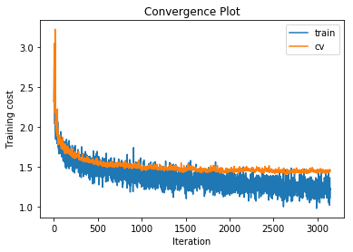
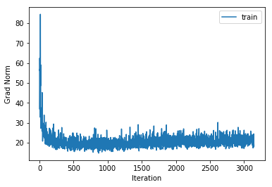
We’ll try a few different architectures. After searching the hyperparameter space a little to find a good learning rate, which I haven’t shown here, we get the following results.
y_train_predicted, cost_train, y_cv_predicted, cost_cv, statistics = \
    train_and_test_fully_connected_neural_network_gradient_descent(
        x_train, y_train, x_cv, y_cv, 0.00, 10, learning_rate=0.001,
        learning_rate_decay=0.95, hidden_sizes=[50],
        num_iterations=10000, max_iterations_without_improvement=500,
        progress_fun=create_progress_bars_and_get_update_fun())

plot_statistics(statistics)

am.print_multiclass_accuracy_measures(y_train_predicted, y_train, cost_train, 'training')
am.print_multiclass_accuracy_measures(y_cv_predicted, y_cv, cost_cv, 'cv')
training  cost  1.21774422602 , accuracy  0.577387755102
cv  cost  1.45697078916 , accuracy  0.483
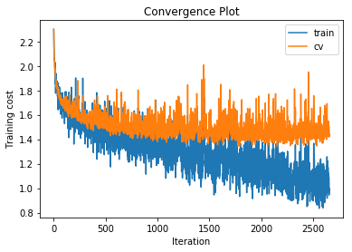
With a single hidden layer with just 50 units we can already increase the accuracy on the cross validation set to 48.3%. What happens if we increase the number of hidden units to 500?
y_train_predicted, cost_train, y_cv_predicted, cost_cv, statistics = \
    train_and_test_fully_connected_neural_network_gradient_descent(
        x_train, y_train, x_cv, y_cv, 0.00, 10, learning_rate=0.002,
        learning_rate_decay=0.95, hidden_sizes=[500],
        num_iterations=10000, max_iterations_without_improvement=500,
        progress_fun=create_progress_bars_and_get_update_fun())

plot_statistics(statistics)

am.print_multiclass_accuracy_measures(y_train_predicted, y_train, cost_train, 'training')
am.print_multiclass_accuracy_measures(y_cv_predicted, y_cv, cost_cv, 'cv')
training  cost  1.06798738968 , accuracy  0.634714285714
cv  cost  1.53666548575 , accuracy  0.503
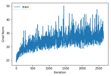
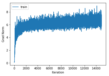
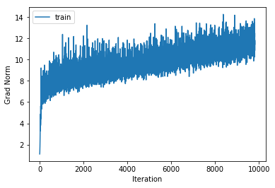
The training accuracy increases alot but the cross validation accuracy only increases by a couple of percentage points, indicating that we are beginning to overfit to the training data. Also note that the gradient norm increases over the course of training indicating that we are not settling into a local minimum. Nonetheless the training cost does converge. This is a known phenomenon which is for example mentioned in the Deep Learning Book.
y_train_predicted, cost_train, y_cv_predicted, cost_cv, statistics = \
    train_and_test_fully_connected_neural_network_gradient_descent(
        x_train, y_train, x_cv, y_cv, 0.00, 10, learning_rate=0.015,
        learning_rate_decay=0.95, hidden_sizes=[50, 50],
        num_iterations=10000, max_iterations_without_improvement=500,
        progress_fun=create_progress_bars_and_get_update_fun())

plot_statistics(statistics)

am.print_multiclass_accuracy_measures(y_train_predicted, y_train, cost_train, 'training')
am.print_multiclass_accuracy_measures(y_cv_predicted, y_cv, cost_cv, 'cv')
training  cost  1.15744138064 , accuracy  0.58687755102
cv  cost  1.43405519542 , accuracy  0.516
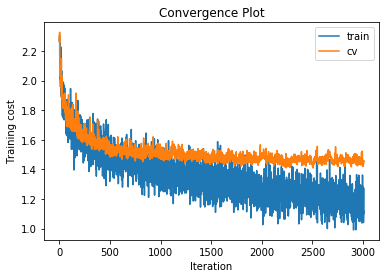
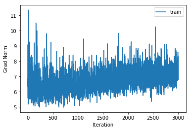
With fewer overall hidden units but a deeper network we get slightly improved performance. This is in line with current research.
y_train_predicted, cost_train, y_cv_predicted, cost_cv, statistics = \
    train_and_test_fully_connected_neural_network_gradient_descent(
        x_train, y_train, x_cv, y_cv, 0.00, 10, learning_rate=0.015,
        learning_rate_decay=0.95, hidden_sizes=[500, 500],
        num_iterations=10000, max_iterations_without_improvement=500,
        progress_fun=create_progress_bars_and_get_update_fun())

plot_statistics(statistics)

am.print_multiclass_accuracy_measures(y_train_predicted, y_train, cost_train, 'training')
am.print_multiclass_accuracy_measures(y_cv_predicted, y_cv, cost_cv, 'cv')
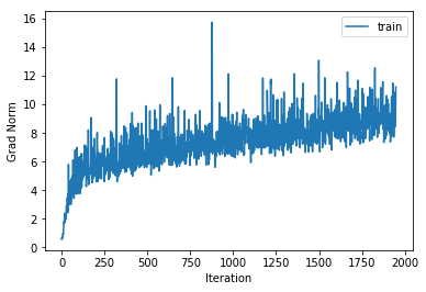
training  cost  0.996452649063 , accuracy  0.655428571429
cv  cost  1.34983136876 , accuracy  0.548
y_train_predicted, cost_train, y_cv_predicted, cost_cv, statistics = \
    train_and_test_fully_connected_neural_network_gradient_descent(
        x_train, y_train, x_cv, y_cv, 0.00, 10, learning_rate=0.06,
        learning_rate_decay=0.95, hidden_sizes=[500, 500, 500],
        num_iterations=10000, max_iterations_without_improvement=500,
        progress_fun=create_progress_bars_and_get_update_fun())

plot_statistics(statistics)

am.print_multiclass_accuracy_measures(y_train_predicted, y_train, cost_train, 'training')
am.print_multiclass_accuracy_measures(y_cv_predicted, y_cv, cost_cv, 'cv')
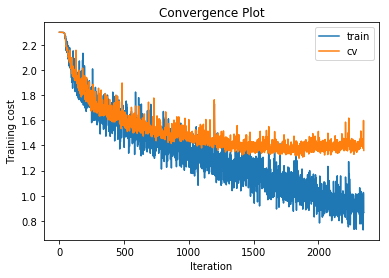
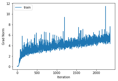
training  cost  0.885157846242 , accuracy  0.68987755102
cv  cost  1.34114145308 , accuracy  0.549
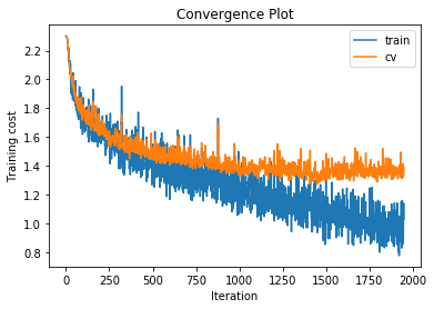
Increasing the number of hidden layers to 3 with 500 units per layer gives very little performance increase over the 2 hidden layer version and leads to increased overfitting.
y_train_predicted, cost_train, y_cv_predicted, cost_cv, statistics = \
    train_and_test_fully_connected_neural_network_gradient_descent(
        x_train, y_train, x_cv, y_cv, 0.00, 10, learning_rate=0.12,
        learning_rate_decay=0.95, hidden_sizes=[500, 500, 500, 500],
        num_iterations=10000, max_iterations_without_improvement=500,
        progress_fun=create_progress_bars_and_get_update_fun())

plot_statistics(statistics)

am.print_multiclass_accuracy_measures(y_train_predicted, y_train, cost_train, 'training')
am.print_multiclass_accuracy_measures(y_cv_predicted, y_cv, cost_cv, 'cv')
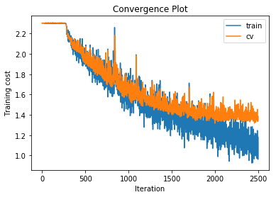
training  cost  1.12007435306 , accuracy  0.598551020408
cv  cost  1.43807103777 , accuracy  0.509
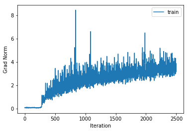
Increasing the number of hidden layers to 4 actually starts to decrease the performance. There is also an interesting effect where the training takes a few hundred iterations to get started.
We now have some higher capacity models but unfortunately this is overfitting to the training data. There are many regularisation strategies we can try. One popular technique for regularisation is to use dropout in which we set some proportion of the node activations to 0 in each forward pass whilst the remaining node activations are scaled up to on average keep the overall output the same.
y_train_predicted, cost_train, y_cv_predicted, cost_cv, statistics = \
    train_and_test_fully_connected_neural_network_gradient_descent(
        x_train, y_train, x_cv, y_cv, 0.00, 10, learning_rate=0.015,
        learning_rate_decay=0.95, hidden_sizes=[500, 500],
        num_iterations=20000, max_iterations_without_improvement=1000,
        dropout_probs=[0.5, 0.5],
        progress_fun=create_progress_bars_and_get_update_fun())

plot_statistics(statistics)

am.print_multiclass_accuracy_measures(y_train_predicted, y_train, cost_train, 'training')
am.print_multiclass_accuracy_measures(y_cv_predicted, y_cv, cost_cv, 'cv')
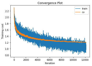
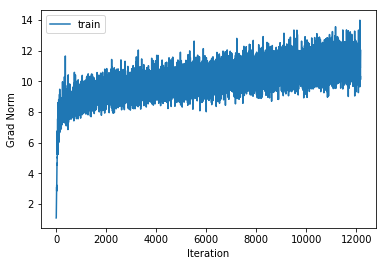
training  cost  0.853029812508 , accuracy  0.733571428571
cv  cost  1.2007222038 , accuracy  0.573
y_train_predicted, cost_train, y_cv_predicted, cost_cv, statistics = \
    train_and_test_fully_connected_neural_network_gradient_descent(
        x_train, y_train, x_cv, y_cv, 0.00, 10, learning_rate=0.06,
        learning_rate_decay=0.95, hidden_sizes=[500, 500, 500],
        num_iterations=20000, max_iterations_without_improvement=1000,
        dropout_probs=[0.5, 0.5, 0.5],
        progress_fun=create_progress_bars_and_get_update_fun())

plot_statistics(statistics)

am.print_multiclass_accuracy_measures(y_train_predicted, y_train, cost_train, 'training')
am.print_multiclass_accuracy_measures(y_cv_predicted, y_cv, cost_cv, 'cv')
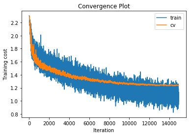
training  cost  0.91532298572 , accuracy  0.708428571429
cv  cost  1.23577688219 , accuracy  0.574
y_train_predicted, cost_train, y_cv_predicted, cost_cv, statistics = \
    train_and_test_fully_connected_neural_network_gradient_descent(
        x_train, y_train, x_cv, y_cv, 0.00, 10, learning_rate=0.1,
        learning_rate_decay=0.95, hidden_sizes=[500, 500, 500, 500],
        num_iterations=20000, max_iterations_without_improvement=1000,
        dropout_probs=[0.5, 0.5, 0.5, 0.5],
        progress_fun=create_progress_bars_and_get_update_fun())

plot_statistics(statistics)

am.print_multiclass_accuracy_measures(y_train_predicted, y_train, cost_train, 'training')
am.print_multiclass_accuracy_measures(y_cv_predicted, y_cv, cost_cv, 'cv')
training  cost  1.10344517089 , accuracy  0.62512244898
cv  cost  1.31410126269 , accuracy  0.533
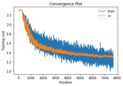
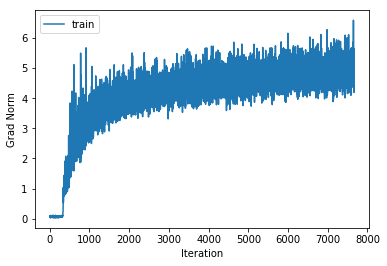
For each of our 3-layer, 4-layer and 5-layer networks this has increased performance on the cross validation set by around 2.5%.
Another thing that we can do is to increase the regularisation strength for the weight decay regularisation mentioned above.
y_train_predicted, cost_train, y_cv_predicted, cost_cv, statistics = \
    train_and_test_fully_connected_neural_network_gradient_descent(
        x_train, y_train, x_cv, y_cv, 0.02, 10, learning_rate=0.015,
        learning_rate_decay=0.95, hidden_sizes=[500, 500],
        num_iterations=20000, max_iterations_without_improvement=1000,
        dropout_probs=[0.5, 0.5],
        progress_fun=create_progress_bars_and_get_update_fun())

plot_statistics(statistics)

am.print_multiclass_accuracy_measures(y_train_predicted, y_train, cost_train, 'training')
am.print_multiclass_accuracy_measures(y_cv_predicted, y_cv, cost_cv, 'cv')
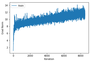
training  cost  1.08335856509 , accuracy  0.685306122449
cv  cost  1.35341525847 , accuracy  0.564
y_train_predicted, cost_train, y_cv_predicted, cost_cv, statistics = \
    train_and_test_fully_connected_neural_network_gradient_descent(
        x_train, y_train, x_cv, y_cv, 0.06, 10, learning_rate=0.015,
        learning_rate_decay=0.95, hidden_sizes=[500, 500],
        num_iterations=20000, max_iterations_without_improvement=1000,
        dropout_probs=[0.5, 0.5],
        progress_fun=create_progress_bars_and_get_update_fun())

plot_statistics(statistics)

am.print_multiclass_accuracy_measures(y_train_predicted, y_train, cost_train, 'training')
am.print_multiclass_accuracy_measures(y_cv_predicted, y_cv, cost_cv, 'cv')
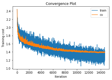
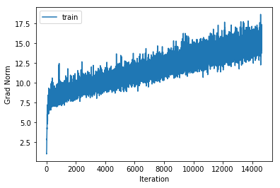
training  cost  1.11365637508 , accuracy  0.69906122449
cv  cost  1.3907269275 , accuracy  0.578
y_train_predicted, cost_train, y_cv_predicted, cost_cv, statistics = \
    train_and_test_fully_connected_neural_network_gradient_descent(
        x_train, y_train, x_cv, y_cv, 0.2, 10, learning_rate=0.015,
        learning_rate_decay=0.95, hidden_sizes=[500, 500],
        num_iterations=20000, max_iterations_without_improvement=1000,
        dropout_probs=[0.5, 0.5],
        progress_fun=create_progress_bars_and_get_update_fun())

plot_statistics(statistics)

am.print_multiclass_accuracy_measures(y_train_predicted, y_train, cost_train, 'training')
am.print_multiclass_accuracy_measures(y_cv_predicted, y_cv, cost_cv, 'cv')
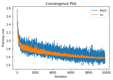
training  cost  1.48631668053 , accuracy  0.565836734694
cv  cost  1.56932527688 , accuracy  0.513
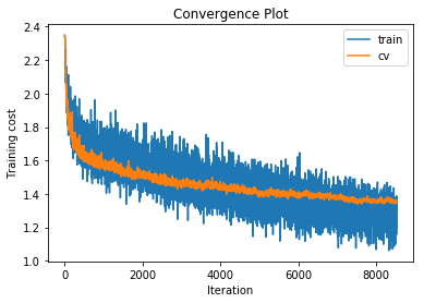
Although a regularisation strength of 0.06 has increased performance by a few tenths of a percent, the lower and higher regularisation strengths decreased performance. For the 4 and 5 layer networks we had similar results and in fact the regularisation strength of 0.06 did not help either. As a result we will leave the regularisation strength set to 0.
To motivate the next regularisation strategy let’s plot learning curves for one of these networks.
plot_learning_curve(x_train, y_train, x_cv, y_cv, 0.00,
                    train_and_test_fully_connected_neural_network_gradient_descent,
                    learning_rate=0.015, learning_rate_decay=0.95, num_iterations=4000,
                    hidden_sizes=[500, 500],
                    progress_fun=create_progress_bars_and_get_update_fun())
training  cost  [ 0.97566225] , accuracy  0.758530612245
cv  cost  [ 1.59021372] , accuracy  0.559
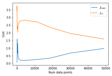
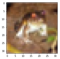
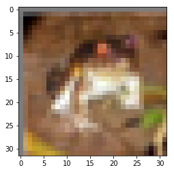
As the number of data points increases the cross validation cost decreases whilst the training cost increases. Since there is still a sizeable gap between the 2 this implies that if we had more data performance on the cross validation set would continue to improve. Since an image of an object is still an image of the same object when translated or rotated a little, we can increase the amount of data we have without gathering any more images by translating images a few pixels and rotating a few degrees.
def translate_and_rotate_image(reshape_to_image, im, max_translation=3, max_rotation_degrees=3):
    '''Given a vector and a function to reshape that data to an image we translate and
    rotate the image by a random amount up to max_translation and max_rotation_degrees
    then flatten the result back into a vector'''
    x_trans = np.random.randint(-max_translation, max_translation)
    y_trans = np.random.randint(-max_translation, max_translation)
    rot = np.random.randint(-max_rotation_degrees, max_rotation_degrees)

    translated = shift(reshape_to_image(im), [y_trans, x_trans, 0])

    rotated = rotate(translated, rot, reshape=False, mode='nearest')
    return rotated.flatten()
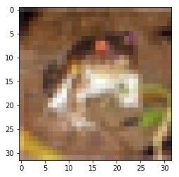
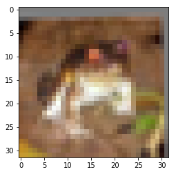
This gives images like the following.
for i in range(4):
    altered_im = translate_and_rotate_image(reshape_to_image, x_train[0,:])
    altered_im -= altered_im.min()
    altered_im /= altered_im.max()
    plt.figure()
    plt.imshow(reshape_to_image(altered_im))
def get_image_alteration(max_translation=3, max_rotation_degrees=3):
    def alter_image(im):
        return translate_and_rotate_image(
            reshape_to_image, im, max_translation=max_translation,
            max_rotation_degrees=max_rotation_degrees)
    return alter_image
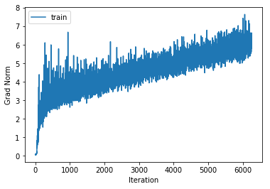
Let’s try this, for example, on the 4-layer neural network with maximum translations of 3 pixels and maximum rotations of 7 degrees.
y_train_predicted, cost_train, y_cv_predicted, cost_cv, statistics = \
    train_and_test_fully_connected_neural_network_gradient_descent(
        x_train, y_train, x_cv, y_cv, 0.00, 10, learning_rate=0.06,
        learning_rate_decay=0.95, hidden_sizes=[500, 500, 500],
        num_iterations=20000, max_iterations_without_improvement=1000,
        alter_data_point=get_image_alteration(3, 7),
        progress_fun=create_progress_bars_and_get_update_fun())

plot_statistics(statistics)

am.print_multiclass_accuracy_measures(y_train_predicted, y_train, cost_train, 'training')
am.print_multiclass_accuracy_measures(y_cv_predicted, y_cv, cost_cv, 'cv')
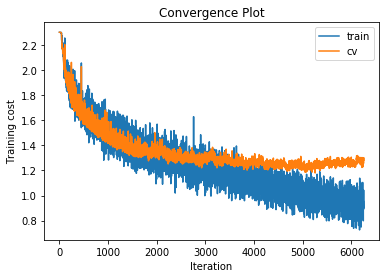
training  cost  0.759427937364 , accuracy  0.729979591837
cv  cost  1.2963962778 , accuracy  0.582
This gives a slightly larger performance improvement compared to using dropout.
